Values

Author

Jay Matsushiba

Published

May 2, 2025

Modified

July 16, 2025

Introduction

This Rmarkdown documents the Zonation5 conservation prioritization analysis used for Bowen Island Biodiversity Planning.

More information on Zonation5

Setup

Code

#### Palen Lab Packages ####
library(bowen.biodiversity.webapp)

#### Other Packages ####
library(here)
library(dplyr)
library(stringr)
library(foreach)
library(sf)
library(terra)
library(tidyterra)
library(readxl)
library(googlesheets4)
library(ggplot2)
library(ggnewscale)
library(RColorBrewer)

sdm_url <- "https://docs.google.com/spreadsheets/d/1IGFwkr9LidcZwbzOJJGSEXLsmpKp0a9gBs65EY-H1xw/edit?usp=sharing"
habitats_url <- "https://docs.google.com/spreadsheets/d/1yDKw4r3tbXYivwtxbbfxc-pYSbtbj_o2ee1pwlNCOO4/edit?usp=drive_link"
output_date <- "2025-06-30"
output_dir <- here("inst/extdata/output_zonation", output_date)

Zonation

Zonation 5 is a spatial prioritization software that can be used to identify priority areas to support conservation planning, land use planning, ecological impact avoidance and other similar tasks. The software uses spatial raster data on the distributions of individual biodiversity features (species, habitats, ecosystem services etc.) to identify which locations in a landscape are most important for retaining biodiversity. Zonation can account for local habitat quality and ecological connectivity together with costs, threats and different land tenure, thus providing a quantitative method for spatial planning that enhances the persistence of biodiversity in the long term.

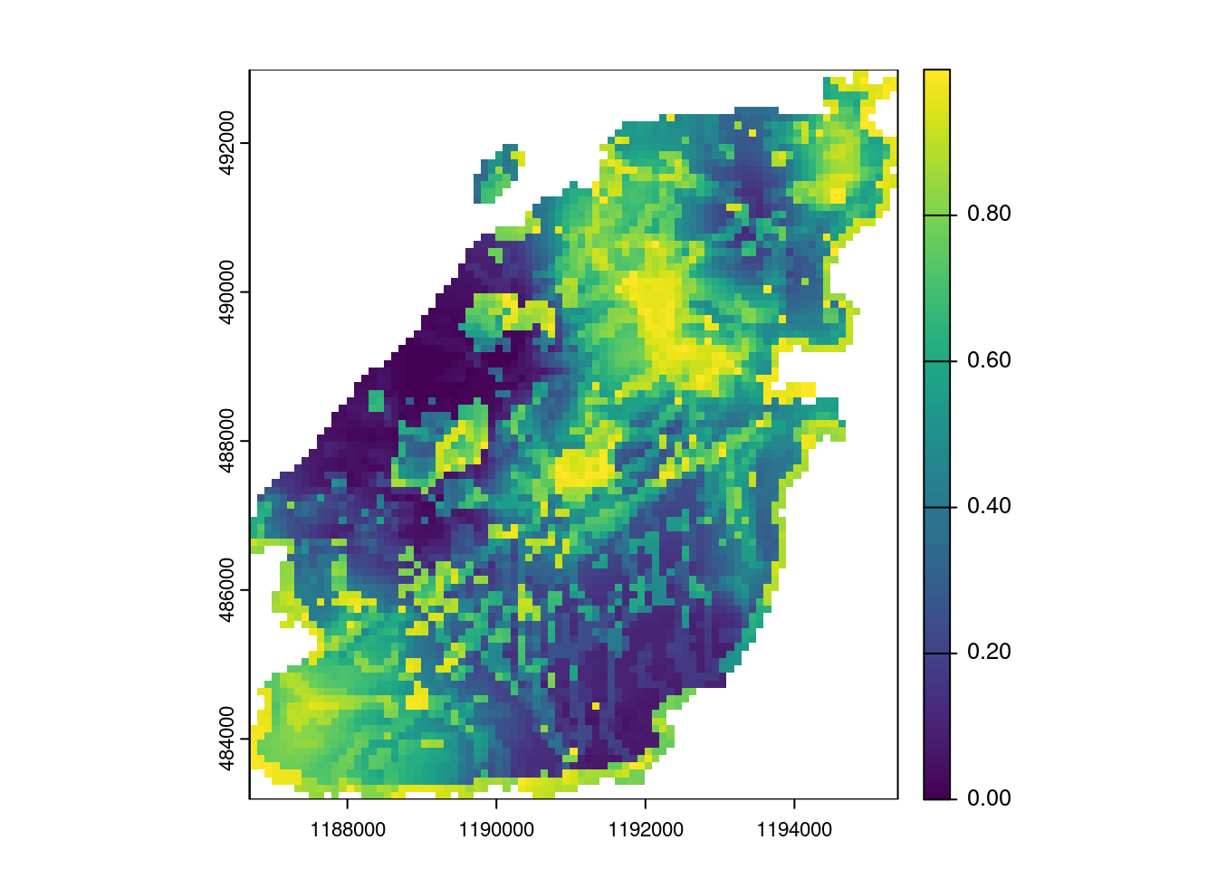
https://zonationteam.github.io/Zonation5/

We took all of the rasters prepared earlier and fed these into the Zonation 5 software. This should provide a relative ranking for locations from highest to lowest for the purposes of biodiversity conservation.

Note: Zonation 5 is usually a standalone application. Here, I have enabled running of Zonation from R, using command line functions. This way we can adjust and automatically run Zonation, reading from data in R.

Check input layers hosted at this link: https://github.com/Palen-Lab/bowen.biodiversity.webapp/tree/main/vignettes/figures/output_zonation_02_05_2025

Information about input layers to the Zonation run here: Habitats - https://docs.google.com/spreadsheets/d/1yDKw4r3tbXYivwtxbbfxc-pYSbtbj_o2ee1pwlNCOO4/edit?gid=1153014884#gid=1153014884 SDMs - https://docs.google.com/spreadsheets/d/1IGFwkr9LidcZwbzOJJGSEXLsmpKp0a9gBs65EY-H1xw/edit?gid=702573996#gid=702573996

Code

#### CREATE DATAFRAME FOR INPUT LAYERS ####
# Read from Google Sheets
habitats_df <- read_sheet(habitats_url, sheet = output_date)
habitats_df$weight <- habitats_df$weight / nrow(habitats_df)
sdm_df <- read_sheet(sdm_url, sheet = output_date) %>%
  select(colnames(habitats_df)) # Select common columns
sdm_df$weight <- sdm_df$weight / nrow(sdm_df)
# Bind all input layers together
layers_df <- bind_rows(habitats_df, sdm_df) %>%
  filter(weight > 0)

# # Check input layers with figure output
# foreach(i=1:nrow(layers_df)) %do% {
#   input_raster <- layers_df[[i, "path"]] %>% rast()
#   bowen_plot <- bowen_map(
#     raster_layer = input_raster,
#     title = layers_df[[i, "name"]],
#     subtitle = paste0(
#       "Category: ", layers_df[[i, "category"]], " ", 
#       "Filepath: ", layers_df[[i, "filename"]], " ", 
#       "Weight: ", layers_df[[i, "weight"]], " ",
#       "Notes: ", layers_df[[i, "notes"]]
#     ),
#     caption = paste0("Source: ", layers_df[[i, "source"]]),
#     legend_label = "value"
#   )
#   figure_output_path <- here("vignettes/figures/output_zonation_02_05_2025/")
#   if(!dir.exists(figure_output_path)) {
#     dir.create(figure_output_path)
#   }
#   ggplot2::ggsave(
#     here(figure_output_path, paste0(tools::file_path_sans_ext(layers_df[[i, "filename"]]), ".png")),
#     bowen_plot,
#     device = ragg::agg_png,
#     width = 9, height = 12, units = "in", res = 300
#   )
# }

Code

#### UPDATE features.txt FOR ZONATION RUN ####
# UPDATE features.txt from files available in data
features_path <- here("vignettes/zonation/features.txt")
cat('"weight" "filename"', 
    file = features_path,
    sep = "\n")
for(i in 1:nrow(layers_df)) {
  next_row <- paste0(layers_df[i, "weight"], " ", layers_df[i, "path"])
  cat(next_row,
      file = features_path,
      append = TRUE,
      sep = "\n")
}
#### SET PARAMS FOR ZONATION RUN ####
zonation5_location <- here("vignettes/zonation/zonation5") 
zonation5_mode <- "CAZ2"
# Zonation5 Setting Text File
zonation5_settings <-  here("vignettes/zonation/settings.z5")
zonation5_settings_txt <- c("feature list file = features.txt", 
                            paste0("analysis area mask layer = ", here("inst/extdata/bowen_mask.tif"))) # Add Bowen Island Mask
writeLines(zonation5_settings_txt, zonation5_settings)
zonation5_output <- here("vignettes/zonation/output") 
zonation5_command <- str_glue(
  '{zonation5_location} -a -w --mode={zonation5_mode} {zonation5_settings} {zonation5_output}',
  zonation5_location = zonation5_location,
  zonation5_mode = zonation5_mode,
  zonation5_settings = zonation5_settings,
  zonation5_output = zonation5_output
) %>%
  str_c()
#### ZONATION RUN ####
system(command = zonation5_command)

#### Save Zonation Run #### 
dir.create(output_dir)
file.copy(list.files(here("vignettes/zonation/output"), full.names = T, recursive = T),
          output_dir,
          recursive = T)

Output

Code

#### VISUALIZE OUTPUT ####
rankmap <- here(output_dir , "rankmap.tif") %>% rast()
plot(rankmap)

Overlap Statistics

Here we calculate the overlap of the top % of conservation values with these other layers:

Protected areas
Private land
Human Footprint (HFP)
Freshwater habitats
- Lakes
- Ponds
- Streams
- Wetlands
- Riparian

Code

# Function for converting Zonation output to boolean based on percentage (in top XX%)
rankmap <- here(output_dir , "rankmap.tif") %>% rast() %>% project(project_crs)

#' Only keep top or bottom cell values by quantile 
#'
#' @param x SpatRaster 
#' @param prob Quantile between 0 and 1
#' @param direction "top" or "bottom", for direction of keep / discard cell values
#'
#' @returns SpatRaster
#' @export
remove_by_quantile <- function(x, prob, direction = "top") {
  val <- x %>%
    values() %>%
    quantile(probs = prob, na.rm = T)
  min_val <- x %>%
    values() %>%
    min(na.rm = T)
  max_val <- x %>%
    values() %>%
    max(na.rm = T)
  if(direction == "top") {
    m <- matrix(c(
      min_val, val, NA,
      val, max_val, 1
    ), ncol = 3, byrow = T)
  } else if (direction == "bottom") {
    m <- matrix(c(
      min_val, val, 1,
      val, max_val, NA
    ), ncol = 3, byrow = T)
  }
  mask_quantile <- x %>%
    classify(m,, include.lowest = T) 
  mask_quantile * x
}

#' Provide ratio of overlap between two rasters (in terms of NA vs nonNA)
#'  
raster_overlap_ratio <- function(top_rast, area_rast) {
  overlap_res <- (top_rast * area_rast)
  top_cell_count <- top_rast %>% terra::global(fun="notNA")
  overlap_cell_count <- overlap_res %>% terra::global(fun="notNA")
  overlap_ratio <- (overlap_cell_count / top_cell_count) %>% as.numeric()
  return(overlap_ratio)
}

# Protected Areas from JD
bowen_protectedareas_rast <- bowen.biodiversity.webapp::bowen_protectedareas %>%
  bowen.biodiversity.webapp::bowen_rasterize()

# Private Land
bowen_mask <- rast(here("inst/extdata/bowen_mask.tif"))
bowen_parcelmap_rast <- bowen.biodiversity.webapp::bowen_parcelmap %>%
  st_cast("MULTIPOLYGON") %>% # Need this due to MULTISURFACE - see: https://gis.stackexchange.com/questions/389814/r-st-centroid-geos-error-unknown-wkb-type-12 
  filter(OwnerType == "Private") %>%
  bowen.biodiversity.webapp::bowen_rasterize()

# Freshwater Habitats 
fw_rast_paths <- c(
  here("inst/extdata/habitats/lakes.tif"),
  here("inst/extdata/habitats/ponds.tif"),
  here("inst/extdata/habitats/riparian.tif"),
  here("inst/extdata/habitats/wetlands.tif"),
  here("inst/extdata/habitats/streams.tif")
)
fw_rast_stack <- lapply(fw_rast_paths, rast) %>%
  rast()
fw_rast_dissolve <- fw_rast_stack %>% 
  sum(na.rm = T) 

# Human Footprint (classified)
bowen_hfp <- here("inst/extdata/habitats/bowen_human_footprint_recl.tif") %>%
  rast()
bowen_hfp_low <- bowen_hfp %>%
  classify(cbind(3, NA)) %>%
  classify(cbind(2, NA))
bowen_hfp_med <- bowen_hfp %>%
  classify(cbind(3, NA)) %>%
  classify(cbind(1, NA))
bowen_hfp_high <- bowen_hfp %>%
  classify(cbind(2, NA)) %>%
  classify(cbind(1, NA))

# Overlap calculation 
overlap_stats <- function(top_rast) {
  data.frame(
    protectedareas_overlap = raster_overlap_ratio(top_rast, bowen_protectedareas_rast),
    privatelands_overlap = raster_overlap_ratio(top_rast, bowen_parcelmap_rast),
    freshwater_overlap = raster_overlap_ratio(top_rast, fw_rast_dissolve),
    hfp_low_overlap = raster_overlap_ratio(top_rast, bowen_hfp_low),
    hfp_med_overlap = raster_overlap_ratio(top_rast, bowen_hfp_med),
    hfp_high_overlap = raster_overlap_ratio(top_rast, bowen_hfp_high)
  )
}

quants <- seq(from = 0, to = 1, by = 0.1)
overlap_results <- foreach(quant = quants, .combine = "rbind") %do% {
  rankmap %>%
    remove_by_quantile(quant) %>%
    overlap_stats() %>% 
    mutate("removed_bottom_quantile" = quant) %>%
    relocate("removed_bottom_quantile")
}
# Visualize output as table for overlap % 
knitr::kable(overlap_results)

removed_bottom_quantile	protectedareas_overlap	privatelands_overlap	freshwater_overlap	hfp_low_overlap	hfp_med_overlap	hfp_high_overlap
0.0	0.3446264	0.5810277	0.4756258	0.0329381	0.6519857	0.3150762
0.1	0.3793392	0.6041405	0.4962359	0.0305312	0.6382267	0.3312422
0.2	0.3780287	0.6184427	0.5088215	0.0183486	0.6334980	0.3481534
0.3	0.3672043	0.6387097	0.5174731	0.0182796	0.6196237	0.3620968
0.4	0.3936637	0.6483689	0.5269762	0.0153701	0.6286073	0.3560226
0.5	0.4136244	0.6605194	0.5333082	0.0112909	0.6398193	0.3488897
0.6	0.4322672	0.6806209	0.5555033	0.0075259	0.6387582	0.3537159
0.7	0.4548306	0.6894605	0.5777917	0.0037641	0.6317440	0.3644918
0.8	0.4553151	0.6782690	0.6114770	0.0037629	0.5879586	0.4082785
0.9	0.5169173	0.6409774	0.6390977	0.0056391	0.5469925	0.4473684
1.0	NaN	NaN	NaN	NaN	NaN	NaN

Overlap Statistics - Polygon on Raster

Here we calculate the overlap of the top % of conservation values with these other layers:

Protected areas
- From John Dowler’s Protected Areas, vs Bowen Island Municipality Protected Areas polygons used for February 1 ver.
- Contains main municipal parks, provincial parks, federal parks (both JD and BIM ver.)
- Addition of covenants, park land exchanges, small municipal parks in JD ver.
- Slightly higher than original February 1 ver. (~18% vs ~21%)
- Protected areas polygons / Bowen Island full polygon (inc. Hutt Island) = 0.2149664
- Protected area extent proportion of Bowen Island using raster method = 0.2189496
Private land
- “Private” - Defined as “Private” in BC ParcelMap polygons
- “Other” - Defined as anything other than “Private” in BC ParcelMap polygons
  - Used to see how much of BC ParcelMap polygons are not Private lands
- Does not add up to 100%, since there are large areas that are not included in BC ParcelMap
- Private lands polygons / Bowen Island full polygon (inc. Hutt Island) = 0.4398566
- Private lands extent proportion of Bowen Island using raster method = 0.4398923
Human Footprint (HFP)
- Proportion of each HFP category (low, medium, high) in the top XX% of biodiversity values
- Should add up to 100%
Freshwater habitats
- Lakes
- Ponds
- Streams
- Wetlands
- Riparian

Code

# Function for converting Zonation output to boolean based on percentage (in top XX%)
rankmap <- here(output_dir , "rankmap.tif") %>% rast() %>% project(project_crs)

#' Only keep top or bottom cell values by quantile 
#'
#' @param x SpatRaster 
#' @param prob Quantile between 0 and 1
#' @param direction "top" or "bottom", for direction of keep / discard cell values
#'
#' @returns SpatRaster
#' @export
remove_by_quantile <- function(x, prob, direction = "top") {
  val <- x %>%
    values() %>%
    quantile(probs = prob, na.rm = T)
  min_val <- x %>%
    values() %>%
    min(na.rm = T)
  max_val <- x %>%
    values() %>%
    max(na.rm = T)
  if(direction == "top") {
    m <- matrix(c(
      min_val, val, NA,
      val, max_val, 1
    ), ncol = 3, byrow = T)
  } else if (direction == "bottom") {
    m <- matrix(c(
      min_val, val, 1,
      val, max_val, NA
    ), ncol = 3, byrow = T)
  }
  mask_quantile <- x %>%
    classify(m,, include.lowest = T) 
  mask_quantile * x
}

#' Rasterize to Bowen Island Mask
bowen_rasterize_cover <- function(sf) {
  bowen_island_mask <- here("inst/extdata/bowen_mask.tif") %>%
    rast() %>%
    project(bowen.biodiversity.webapp::project_crs)

  output <- sf %>%
    terra::vect() %>% # Change to SpatVector for rasterization
    terra::project(bowen.biodiversity.webapp::project_crs) %>% # Reproject to the mask CRS
    terra::rasterize(bowen_island_mask,
                     cover = T, # Return proportion of cell covered by polygon 
                     background = NA) # Rasterize to match mask, set background values to NA
}

#' Provide ratio of overlap between two rasters (in terms of NA vs nonNA)
raster_overlap_ratio <- function(top_rast, area_rast) {
  overlap_res <- (top_rast * area_rast)
  top_cell_count <- top_rast %>% 
    global("sum", na.rm = T)
  overlap_cell_values <- overlap_res %>% 
    values(na.rm = T) 
  overlap_cell_area <-overlap_cell_values %>% sum()
  overlap_ratio <- (overlap_cell_area / top_cell_count) %>% as.numeric()
  return(overlap_ratio)
}

# Bowen entire area
bowen_island <- st_read(here("data-raw/bowen_island_shoreline_w_hutt.gpkg"), layer = "bowen_island_shoreline_w_hutt__bowen_islands")

Reading layer `bowen_island_shoreline_w_hutt__bowen_islands' from data source 
  `/home/jay/Programming_Projects/bowen.biodiversity.webapp/data-raw/bowen_island_shoreline_w_hutt.gpkg' 
  using driver `GPKG'
Simple feature collection with 11 features and 1 field
Geometry type: POLYGON
Dimension:     XY
Bounding box:  xmin: 4001956 ymin: 2020764 xmax: 4013988 ymax: 2028901
Projected CRS: NAD83 / Statistics Canada Lambert

Code

# Protected Areas from JD
bowen_protectedareas_include <- bowen.biodiversity.webapp::bowen_protectedareas %>%
  filter(type != "Agricultural Land Reserve") # Remove ALR
# Protected Areas from Bowen Island Municipality 
bowen_protectedareas_2 <- st_read(here("data-raw/archive/bowen_island_protectedareas/BM_PROTECTED_AREAS.shp")) %>%
  filter(NAME != "Old Growth Management Area")

Reading layer `BM_PROTECTED_AREAS' from data source 
  `/home/jay/Programming_Projects/bowen.biodiversity.webapp/data-raw/archive/bowen_island_protectedareas/BM_PROTECTED_AREAS.shp' 
  using driver `ESRI Shapefile'
Simple feature collection with 61 features and 2 fields
Geometry type: MULTIPOLYGON
Dimension:     XY
Bounding box:  xmin: 468632.2 ymin: 5464739 xmax: 476690.7 ymax: 5472342
Projected CRS: NAD83 / UTM zone 10N

Code

# JD protected areas is more complete, with smaller municipal parks, covenants, and park land exchanges

bowen_protectedareas_rast <- bowen_protectedareas_include %>%
  bowen_rasterize_cover()

# Check with polygon / polygon area calculations for full Bowen Island
sum(st_area(bowen_protectedareas_include)) / sum(st_area(bowen_island)) # 0.2149664

0.2149664 [1]

Code

sum(st_area(bowen_protectedareas_2)) / sum(st_area(bowen_island)) # 0.17935

0.17935 [1]

Code

# Private Land
bowen_mask <- rast(here("inst/extdata/bowen_mask.tif"))
bowen_parcelmap_priv <- bowen.biodiversity.webapp::bowen_parcelmap %>%
  st_cast("MULTIPOLYGON") %>% # Need this due to MULTISURFACE - see: https://gis.stackexchange.com/questions/389814/r-st-centroid-geos-error-unknown-wkb-type-12 
  filter(OwnerType == "Private")
bowen_parcelmap_rast <- bowen_parcelmap_priv %>%
  bowen_rasterize_cover()

# Check with polygon / polygon area calculations for full Bowen Island 
sum(st_area(bowen_parcelmap_priv)) / sum(st_area(bowen_island)) # 0.4398566

0.4398566 [1]

Code

# Other Land
bowen_mask <- rast(here("inst/extdata/bowen_mask.tif"))
bowen_parcelmap_other_rast <- bowen.biodiversity.webapp::bowen_parcelmap %>%
  st_cast("MULTIPOLYGON") %>%# Need this due to MULTISURFACE - see: https://gis.stackexchange.com/questions/389814/r-st-centroid-geos-error-unknown-wkb-type-12 
  filter(OwnerType != "Private") %>%
  bowen_rasterize_cover()

# Freshwater Habitats 
fw_rast_paths <- c(
  here("inst/extdata/habitats/lakes.tif"),
  here("inst/extdata/habitats/ponds.tif"),
  here("inst/extdata/habitats/riparian.tif"),
  here("inst/extdata/habitats/wetlands.tif"),
  here("inst/extdata/habitats/streams.tif")
)
fw_rast_stack <- lapply(fw_rast_paths, rast) %>%
  rast()
fw_rast_dissolve <- fw_rast_stack %>% 
  sum(na.rm = T) %>%
  not.na() %>%
  classify(cbind(FALSE, NA)) 

# Human Footprint (classified)
bowen_hfp <- here("inst/extdata/habitats/bowen_human_footprint_recl.tif") %>%
  rast()
bowen_hfp_low <- bowen_hfp %>%
  classify(cbind(3, NA)) %>%
  classify(cbind(2, NA)) %>%
  not.na() %>%
  classify(cbind(FALSE, NA)) 
bowen_hfp_med <- bowen_hfp %>%
  classify(cbind(3, NA)) %>%
  classify(cbind(1, NA)) %>%
  not.na() %>%
  classify(cbind(FALSE, NA)) 
bowen_hfp_high <- bowen_hfp %>%
  classify(cbind(2, NA)) %>%
  classify(cbind(1, NA)) %>%
  not.na() %>%
  classify(cbind(FALSE, NA)) 

# Overlap calculation 
overlap_stats <- function(top_rast) {
  data.frame(
    protectedareas_overlap = raster_overlap_ratio(top_rast, bowen_protectedareas_rast),
    privatelands_overlap = raster_overlap_ratio(top_rast, bowen_parcelmap_rast),
    otherlands_overlap = raster_overlap_ratio(top_rast, bowen_parcelmap_other_rast),
    freshwater_overlap = raster_overlap_ratio(top_rast, fw_rast_dissolve),
    hfp_low_overlap = raster_overlap_ratio(top_rast, bowen_hfp_low),
    hfp_med_overlap = raster_overlap_ratio(top_rast, bowen_hfp_med),
    hfp_high_overlap = raster_overlap_ratio(top_rast, bowen_hfp_high)
  )
}

quants <- seq(from = 0.9, to = 0, by = -0.1)
overlap_results <- foreach(quant = quants, .combine = "rbind") %do% {
  rankmap %>%
    remove_by_quantile(quant) %>%
    overlap_stats() %>% 
    mutate("top_bioval_prop" = 1-quant) %>%
    relocate("top_bioval_prop") 
}
# Visualize output as table for overlap % 
knitr::kable(overlap_results)

top_bioval_prop	protectedareas_overlap	privatelands_overlap	otherlands_overlap	freshwater_overlap	hfp_low_overlap	hfp_med_overlap	hfp_high_overlap
0.1	0.3174649	0.3945937	0.2928323	0.6387667	0.0055659	0.5481426	0.4462914
0.2	0.2647937	0.4394002	0.2660174	0.6126650	0.0038225	0.5859312	0.4102463
0.3	0.2626128	0.4703340	0.2489584	0.5831383	0.0037686	0.6252945	0.3709370
0.4	0.2485606	0.4735271	0.2376814	0.5641232	0.0067621	0.6326465	0.3605914
0.5	0.2409733	0.4664929	0.2377358	0.5465734	0.0095868	0.6342642	0.3561491
0.6	0.2304698	0.4625577	0.2359358	0.5410867	0.0124238	0.6278010	0.3597752
0.7	0.2200468	0.4605420	0.2301998	0.5348029	0.0142620	0.6228655	0.3628725
0.8	0.2235007	0.4550586	0.2259611	0.5307384	0.0145557	0.6280725	0.3573717
0.9	0.2253763	0.4524188	0.2228878	0.5272985	0.0176638	0.6297194	0.3526168
1.0	0.2234341	0.4512389	0.2218854	0.5247490	0.0179839	0.6310762	0.3509399