Habitats

Author

Jay Matsushiba

Published

April 25, 2025

Introduction

This page describes the preparing of habitat layers for input into the Zonation5 conservation prioritization software.

Setup

Code

library(bowen.biodiversity.webapp)
library(here)
library(sf)
library(tidyverse)
library(terra)
library(leaflet)
library(googlesheets4)

# Load Bowen Island Mask Created Previously
bowen_island_mask <- here("inst/extdata/bowen_mask.tif") %>%
  rast() %>%
  project(project_crs)

# Rasterize to Bowen Island Mask 
bowen_rasterize <- function(sf) {
  output <- sf %>% 
    terra::vect() %>% # Change to SpatVector for rasterization
    terra::project(project_crs) %>% # Reproject to the mask CRS
    terra::rasterize(bowen_island_mask,
                     touches = T,
                     background = NA) # Rasterize to match mask, set background values to NA
}

# Path for this vignette's outputs
output_path <- here("inst/extdata/habitats")

# Habitats table 
habitats_df <- data.frame(
  path = as.character(),
  filename = as.character(),
  name = as.character(),
  weight = as.numeric(),
  category = as.character(),
  source = as.character(),
  notes = as.character()
)

Metro Vancouver Sensitive Ecosystem Inventory

Previously, for the Feb 1 2025 workshop, we used the Sensitive Ecosystem Inventory from Metro Vancouver. These habitat types were originally represented as polygon areas, which was converted to raster.

Code

#### Metro Vancouver Sensitive Ecosystems Inventory ####
# Contents of "data-raw/metrovancouver_sensitive_ecosystem_inventory/" downloaded from MetroVancouver Open Data Catalogue
# GeoPackage download: https://arcg.is/TnfXL 
# Reports download: https://metrovancouver.org/services/regional-planning/sensitive-ecosystem-inventory-mapping-app
mvsei <- st_read(here("data-raw/metrovancouver_sensitive_ecosystem_inventory/Sensitive_Ecosystem_Inventory_for_Metro_Vancouver__2020__-5580727563910851507.gpkg")) %>%
  st_transform(crs = bowen.biodiversity.webapp::project_crs)

Reading layer `Sensitive_Ecosystem_Inventory_for_Metro_Vancouver__2020_' from data source `/home/jay/Programming_Projects/bowen.biodiversity.webapp/data-raw/metrovancouver_sensitive_ecosystem_inventory/Sensitive_Ecosystem_Inventory_for_Metro_Vancouver__2020__-5580727563910851507.gpkg' 
  using driver `GPKG'
Simple feature collection with 25637 features and 99 fields
Geometry type: MULTIPOLYGON
Dimension:     XYZ
Bounding box:  xmin: 468516.6 ymin: 5427679 xmax: 547072.5 ymax: 5495732
z_range:       zmin: 0 zmax: 0
Projected CRS: NAD83 / UTM zone 10N

Code

mvsei_secl_codes <- read.csv(here("data-raw/metrovancouver_sensitive_ecosystem_inventory/SEI_SECl_codes.csv"))
mvsei_sesubcl_codes <- read.csv(here("data-raw/metrovancouver_sensitive_ecosystem_inventory/SEI_SEsubcl_codes.csv"))

# Bowen Island SEI 
bowen_sei <- mvsei %>% 
  st_intersection(st_as_sf(bowen.biodiversity.webapp::bowen_boundary))

Warning: attribute variables are assumed to be spatially constant throughout
all geometries

Wetlands

There were some areas identified as potentially incorrect during the Feb 1 2025 workshop. We followed up with Alan Whitehead and John Dowler via email for additional details. See issue here: Link

Alan Whitehead provided ponds and wetlands shapefiles, that he had created over the years as an environmental consultant on Bowen Island.

In the first Zonation run, we combined WN for both SECl_1 and SECl_2. This overestimated wetland extent, since this included areas that were more likely to have another habitat quality based off of MV methodology (which was mostly based on aerial surveys). We also pulled out the “Shallow Water” subcategory into its seperate layer.

For this next Zonation run, we will use the wetlands layer provided by Alan Whitehead. This layer seemed to be more complete with ground-truthing of the location of these wetlands, in comparison to the SEI layers from MetroVancouver that were verified using aerial imagery. “Shallow Water” is no longer a separate habitat type, since Alan Whitehead’s layers do not provide this classification.

Code

# Alan Whitehead's Wetland Layer
wetlands_aw <- bowen.biodiversity.webapp::bowen_wetlands_whitehead_consultants
# Bowen SEI SECl_1 
bowen_sei_wn_1 <- bowen_sei %>%
  filter(SECl_1 == "WN")
# Bowen SEI SECl_2
bowen_sei_wn_2 <- bowen_sei %>%
  filter(SECl_2 == "WN")

wetlands_aw_rast <- bowen_rasterize(wetlands_aw)
bowen_sei_wn_1_rast <- bowen_rasterize(bowen_sei_wn_1)
bowen_sei_wn_2_rast <- bowen_rasterize(bowen_sei_wn_2)

# Compare wetlands 
leaflet(width = "100%", height = "800px") %>%
  addProviderTiles(provider = providers$Stadia.AlidadeSmooth) %>%
  addRasterImage(x = wetlands_aw_rast, group = "A. Whitehead Wetlands", colors = "green") %>%
  addPolygons(data = st_transform(wetlands_aw, 4326), group = "A. Whitehead Wetlands", color = "darkgreen") %>%
  addRasterImage(x = bowen_sei_wn_1_rast, group = "Bowen SEI SECl_1 Wetlands", colors = "blue") %>%
  addPolygons(data = st_transform(bowen_sei_wn_1, 4326), group = "Bowen SEI SECl_1 Wetlands", color = "darkblue") %>%
  addRasterImage(x = bowen_sei_wn_2_rast, group = "Bowen SEI SECl_2 Wetlands", colors = "orange") %>%
  addPolygons(data = st_transform(bowen_sei_wn_2, 4326), group = "Bowen SEI SECl_2 Wetlands", color = "darkorange") %>%
  addLayersControl(overlayGroups = c("A. Whitehead Wetlands", 
                                     "Bowen SEI SECl_1 Wetlands", 
                                     "Bowen SEI SECl_2 Wetlands"
  ),
  options = layersControlOptions(collapsed = F))

Code

# Output 
writeRaster(wetlands_aw_rast, here(output_path, "wetlands.tif"), overwrite = T)
habitats_df <- data.frame(
  path = here(output_path, "wetlands.tif"),
  filename = "wetlands.tif",
  name = "Wetlands",
  weight = 1.0,
  category = "Freshwater",
  source = "Alan Whitehead",
  notes = "replaces MVSEI"
) %>%
  bind_rows(habitats_df)

Freshwater

The initial Feb1 Zonation run used the SEI categories to represent freshwater ecosystems. Each subcategory of freshwater was used as a distinct layer in the Zonation run. We have since acquired some new layers, which we can simply convert to raster and include as a conservation value input to start.

Alan Whitehead’s Ponds layer seems much more complete than what is available in SEI, so we will use that instead to create the habitat layer.

Code

#### Ponds ####
# Create Ponds Layer from Alan Whitehead's Map and SEI Freshwaster Ponds
ponds_aw <- bowen.biodiversity.webapp::bowen_ponds_whitehead_consultants
ponds_aw

Simple feature collection with 122 features and 7 fields
Geometry type: MULTIPOLYGON
Dimension:     XY
Bounding box:  xmin: 469230.7 ymin: 5464929 xmax: 476786.3 ymax: 5473554
Projected CRS: NAD83 / UTM zone 10N
First 10 features:
   ID    Area                  NAME
1  66  196.48       Everhard's Pond
2  67  701.58        Trethewey Pond
3  42  793.69           Ballou Pond
4  78   84.99              un named
5  79  416.44                island
6  80  183.33              un named
7  72 2701.43 Little Josephine Lake
8  36 3962.48          Macleod Pond
9  37 1761.08     Upper Quarry Pond
10 69  816.51           Carter Pond
                                            COMMENT                 OCP_CLASS
1                          constructed private pond          non-fish bearing
2                          constructed private pond          non-fish bearing
3                          constructed private pond          non-fish bearing
4                          constructed private pond          non-fish bearing
5     island in constructed pond FID43; fix polygon                      <NA>
6                          constructed private pond          non-fish bearing
7  constructed private pond, hist. w/ stocked trout tributary to fish-fearing
8                   constructed pond, former quarry tributary to fish-bearing
9                   constructed pond, former quarry tributary to fish-bearing
10     in Terminal Creek, water source for hatchery              fish-bearing
   Source Perimeter                           geom
1    <NA>        52 MULTIPOLYGON (((474905.9 54...
2    <NA>        97 MULTIPOLYGON (((475005 5470...
3    <NA>       146 MULTIPOLYGON (((474696.6 54...
4    <NA>        57 MULTIPOLYGON (((470954.3 54...
5      AW        76 MULTIPOLYGON (((471305.8 54...
6    <NA>        52 MULTIPOLYGON (((471427.8 54...
7    <NA>       477 MULTIPOLYGON (((472313.9 54...
8    <NA>       355 MULTIPOLYGON (((471303.8 54...
9    <NA>       163 MULTIPOLYGON (((471181.1 54...
10   <NA>        72 MULTIPOLYGON (((474527 5469...

Code

# Source for ponds is Islands Trust TEM
bowen_sei_fw_pd <- bowen_sei %>%
  filter(SEsubcl_1 == "pd" | SEsubcl_2 == "pd") %>%
  st_transform(st_crs(ponds_aw))
# Ponds Rasters 
ponds_aw_rast <- bowen_rasterize(ponds_aw)
bowen_sei_fw_pd_rast <- bowen_rasterize(bowen_sei_fw_pd)
# Compare ponds 
leaflet(width = "100%", height = "800px") %>%
  addProviderTiles(provider = providers$Stadia.AlidadeSmooth) %>%
  addRasterImage(x = ponds_aw_rast, group = "A. Whitehead Ponds", colors = "green") %>%
  addPolygons(data = st_transform(ponds_aw, 4326), group = "A. Whitehead Ponds", color = "darkgreen") %>%
  addRasterImage(x = bowen_sei_fw_pd_rast, group = "Bowen SEI Ponds", colors = "blue") %>%
  addPolygons(data = st_transform(bowen_sei_fw_pd, 4326), group = "Bowen SEI Ponds", color = "darkblue") %>%
  addLayersControl(overlayGroups = c("A. Whitehead Ponds", 
                                     "Bowen SEI Ponds"
  ),
  options = layersControlOptions(collapsed = F))

Code

# Save AW ponds
writeRaster(ponds_aw_rast, here(output_path, "ponds.tif"), overwrite = T)
habitats_df <- data.frame(
  path = here(output_path, "ponds.tif"),
  filename = "ponds.tif",
  name = "Ponds",
  weight = 1.0,
  category = "Freshwater",
  source = "Alan Whitehead",
  notes = "replaces MVSEI"
) %>%
  bind_rows(habitats_df)
#### Lakes ####
bowen_sei_fw_la_rast <- bowen_sei %>%
  filter(SEsubcl_1 == "la" | SEsubcl_2 == "la") %>%
  bowen_rasterize()
writeRaster(bowen_sei_fw_la_rast, here(output_path, "lakes.tif"), overwrite = T)
habitats_df <- data.frame(
  path = here(output_path, "lakes.tif"),
  filename = "lakes.tif",
  name = "Lakes",
  weight = 1.0,
  category = "Freshwater",
  source = "MVSEI",
  notes = ""
) %>%
  bind_rows(habitats_df)

#### Fish Bearing Streams ####
# Create separate raster for each OCP class
streams_fishbearing_rast <- bowen.biodiversity.webapp::bowen_fish_whitehead_consultants %>%
  filter(OCP_CLASS == "fish-bearing") %>%
  bowen_rasterize() %>%
  classify(matrix(c(1, 3), ncol = 2, byrow = T)) # Assign value 3 
streams_tributary_rast <- bowen.biodiversity.webapp::bowen_fish_whitehead_consultants %>%
  filter(OCP_CLASS == "tributary to fish-bearing") %>%
  bowen_rasterize() %>%
  classify(matrix(c(1, 2), ncol = 2, byrow = T)) # Assign value 2
streams_nonfishbearing_rast <- bowen.biodiversity.webapp::bowen_fish_whitehead_consultants %>%
  filter(OCP_CLASS == "non-fish bearing") %>%
  bowen_rasterize() %>%
  classify(matrix(c(1, 1), ncol = 2, byrow = T)) # Assign value 1
streams_drainage_rast <- bowen.biodiversity.webapp::bowen_fish_whitehead_consultants %>%
  filter(OCP_CLASS == "drainage channel") %>% 
  bowen_rasterize() %>% 
  classify(matrix(c(1, 1), ncol = 2, byrow = T)) # Assign value 1
streams_NA_rast <- bowen.biodiversity.webapp::bowen_fish_whitehead_consultants %>%
  filter(is.na(OCP_CLASS)) %>%
  bowen_rasterize() %>%
  classify(matrix(c(1, 1), ncol = 2, byrow = T)) # Assign value 1
# Combine stream rasters together, cover in order of importance
streams_rast <- streams_NA_rast %>%
  cover(streams_drainage_rast) %>%
  cover(streams_nonfishbearing_rast) %>%
  cover(streams_tributary_rast) %>%
  cover(streams_fishbearing_rast)
writeRaster(streams_rast, here(output_path, "streams.tif"), overwrite = T)
habitats_df <- data.frame(
  path = here(output_path, "streams.tif"),
  filename = "streams.tif",
  name = "Streams",
  weight = 1.0,
  category = "Freshwater",
  source = "Alan Whitehead",
  notes = "Raster value 3 for fish-bearing streams, 2 for non-fish bearing, 1 for drainage channel and NA"
) %>%
  bind_rows(habitats_df)

#### Riparian #### 
# Combine ff (fringe) and gu (gully) riparian classes into one habitat layer
bowen_sei_ri_rast <- bowen_sei %>%
  filter(SECl_1 == "RI" | SECl_2 == "RI") %>%
  bowen_rasterize()
writeRaster(bowen_sei_ri_rast, here(output_path, "riparian.tif"), overwrite = T)
habitats_df <- data.frame(
  path = here(output_path, "riparian.tif"),
  filename = "riparian.tif",
  name = "Riparian",
  weight = 1.0,
  category = "Freshwater",
  source = "MVSEI",
  notes = ""
) %>%
  bind_rows(habitats_df)

Terrestrial Ecosystem Mapping

We originally used the Metro Vancouver SEI for the Feb 1 Zonation run, but many of the habitat types are not very specific. Ex. “Mature Forest” is a habitat category that covers much of Bowen Island, but does not provide detail of what species exist there.

We got the TEM (Terrestrial Ecosystem Mapping) layers from Jeff Matheson via email on April 6 2025.

From my own digging through the MVSEI layers and comparing to the TEM, I think that the original 2009 version of the TEMs are included in the current MVSEI. Since then TEM has been updated (2011 and 2017), mostly with larger polygons being split into smaller and more specific areas, but these have not been incorporated into MVSEI. The most recent additions to MVSEI from the TEM are in 2016, before the most recent updates.

Code

#### Bowen TEM for detailed terrestrial habitat identity ####
bowen_TEM <- st_read(here("data-raw/bowen_TEM/BM_TEM.shp")) %>%
  # Remove habitat types that are already represented or not important ecosystems
  filter(!SITE_S1_LA %in% c(
    # Freshwater  
    "Reservoir",
    "Shallow Open Water",
    "Lake",
    # Developed 
    "Gravel Pit",
    "Cultivated Field",
    "Golf Course",
    "Rural",
    "Industrial",
    "Urban/Suburban",
    # Wetlands - already represented in A.Whitehead's layers
    "Wetland swamp",
    "Wetland fenn"
    )
  )

Reading layer `BM_TEM' from data source 
  `/home/jay/Programming_Projects/bowen.biodiversity.webapp/data-raw/bowen_TEM/BM_TEM.shp' 
  using driver `ESRI Shapefile'
Simple feature collection with 615 features and 43 fields
Geometry type: POLYGON
Dimension:     XY
Bounding box:  xmin: 468516.6 ymin: 5464606 xmax: 477662.2 ymax: 5474194
Projected CRS: NAD83 / UTM zone 10N

Code

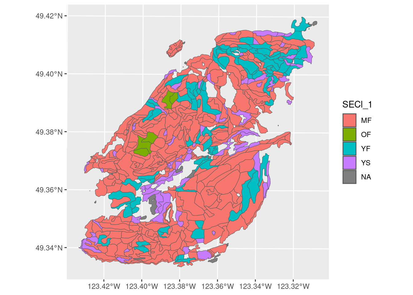
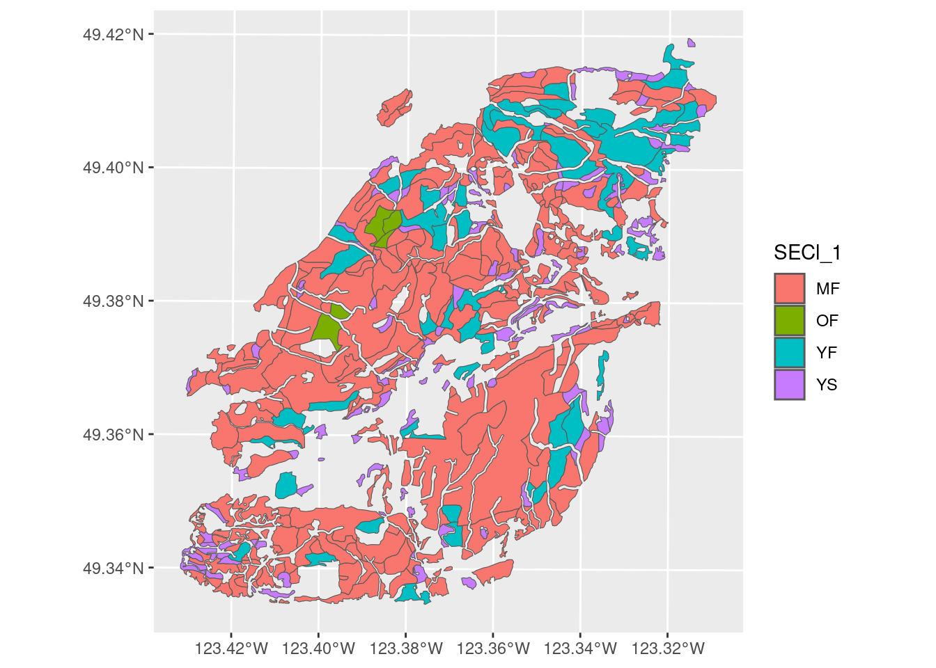
# Create rasters and save
bowen_TEM_categories <- unique(bowen_TEM$SITE_S1_LA)
for(tem_code in bowen_TEM_categories) {
  output <- bowen_TEM[bowen_TEM$SITE_S1_LA == tem_code,] %>%
    bowen_rasterize()
  output_filename <- tem_code %>% 
    gsub("-", "_", .) %>%
    gsub(" ", "", .) %>%
    gsub("'", "", .) %>%
    paste0(".tif")
  writeRaster(output, here(output_path, output_filename), overwrite = T)
  habitats_df <- data.frame(
    path = here(output_path, output_filename),
    filename = output_filename,
    name = tem_code,
    weight = 1.0,
    category = "Terrestrial",
    source = "TEM",
    notes = "Detailed types, plant community descriptions"
  ) %>%
    bind_rows(habitats_df)
}

#### Metro Vancouver SEI for Young Forest, Mature Forest, Old Forest designation ####
# OF - Old Forest
# MF - Mature Forest
# YF - Young Forest
# YS - Young Forest (Small)
bowen_SEI_forests <- bowen_sei %>%
  select(SECl_1) %>%
  filter(SECl_1 %in% c("OF", "MF", "YF", "YS")) %>%
  st_transform(st_crs(bowen_TEM))
bowen_TEM_forests <- bowen_sei %>%
  select(SECl_1) %>%
  filter(SECl_1 %in% c("OF", "MF", "YF", "YS")) %>%
  st_transform(st_crs(bowen_TEM)) %>%
  st_join(bowen_TEM, ., largest = T) # Spatial join by largest, so each TEM polygon has forest category

Warning: attribute variables are assumed to be spatially constant throughout
all geometries

Code

# Compare forest maps to check
ggplot(bowen_TEM_forests) + geom_sf(aes(fill = SECl_1))

Code

ggplot(bowen_SEI_forests) + geom_sf(aes(fill = SECl_1))

Code

# Create rasters and save
bowen_forest_categories <- unique(bowen_TEM_forests$SECl_1) 
bowen_forest_categories <- bowen_forest_categories[!is.na(bowen_forest_categories)]
for(category in bowen_forest_categories) {
  output <- bowen_TEM_forests[bowen_TEM_forests$SECl_1 == category,] %>%
    bowen_rasterize()
  output_filename <- category %>% 
    gsub("-", "_", .) %>%
    gsub(" ", "", .) %>%
    gsub("'", "", .) %>%
    paste0(".tif")
  writeRaster(output, here(output_path, output_filename), overwrite = T)
  habitats_df <- data.frame(
    path = here(output_path, output_filename),
    filename = output_filename,
    name = category,
    weight = 1.0,
    category = "Terrestrial",
    source = "MVSEI",
    notes = mvsei_secl_codes[mvsei_secl_codes$code == category, "description"]
  ) %>%
    bind_rows(habitats_df)
}

# Metro Vancouver SEI for coastal areas - intertidal (IT), herbaceous (HB)
bowen_sei_no_tem <- bowen_sei %>%
  filter(!ProjType == "TEM" & !ProjType == "NEM") %>%
  # Remove polygons with SECl x__, because these are lost ecosystem areas 
  filter(!SECl_1 %in% c("xRI", "xWD", "xMF")) %>%
  # Remove polygons with these SEsubcl, since represented elsewhere
  # co conifer dominated
  # ff riparian fringe
  # sp swamp
  # sw shallow water
  # mx mixed confider broadleaf
  filter(!SEsubcl_1 %in% c("co", "ff", "sp", "sw", "mx")) 

bowen_sei_no_tem_categories <- bowen_sei_no_tem$SEsubcl_1 %>% unique()
for(category in bowen_sei_no_tem_categories) {
  output <- bowen_sei_no_tem[bowen_sei_no_tem$SEsubcl_1 == category,] %>%
    bowen_rasterize()
  output_filename <- category %>% 
    gsub("-", "_", .) %>%
    gsub(" ", "", .) %>%
    gsub("'", "", .) %>%
    paste0(".tif")
  writeRaster(output, here(output_path, output_filename), overwrite = T)
  habitats_df <- data.frame(
    path = here(output_path, output_filename),
    filename = output_filename,
    name = category,
    weight = 1.0,
    category = "Terrestrial",
    source = "MVSEI",
    notes = mvsei_sesubcl_codes[mvsei_sesubcl_codes$SEsubcl == category, "description"]
  ) %>%
    bind_rows(habitats_df)
}

Bowen Heron Watch

Data on Heron and Raptor nest sites on Bowen Island from Carla Skuce on Feb 4 2025.

Challenges:

No common ID between Excel spreadsheet and shapefile point locations

Addressed by manually looking up location description on Google Maps and matching to points in QGIS. For some points, I created new points that matched the location description. I figured at the 100 m resolution that we are working with, the precise location would not be that necessary.

Due to sensitivity of this data, this layer will not be provided or mapped on its own.

Code

#### Heron Nests ####
# This geopackage was created in QGIS with manual matching between excel spreadsheet and shapefile provided from Bowen Heron Watch
bowen_heron_watch <- st_read(here("data-raw/bowen_heron_watch/bowen_heron_watch.gpkg")) 
# Replace NAs
bowen_heron_watch[is.na(bowen_heron_watch)] <- 0 
bowen_heron_watch$bowen_heron_watch_2018 <- as.numeric(bowen_heron_watch$bowen_heron_watch_2018)
# Summarize - total nests all time
bowen_heron_watch$total <- bowen_heron_watch[,6:31] %>%
  st_drop_geometry() %>%
  rowSums()
# Rasterize the heron sites 
bowen_heron_nest_rast <- bowen_heron_watch %>%
  vect() %>% 
  project(bowen_island_mask) %>%
  rasterize(bowen_island_mask, field = "total", fun = sum, cover = T, touches = T) 
plot(bowen_heron_nest_rast)

Code

writeRaster(bowen_heron_nest_rast, here(output_path, "bowen_heron_nest.tif"), overwrite = T)
habitats_df <- data.frame(
    path = here(output_path, "bowen_heron_nest.tif"),
    filename = "bowen_heron_nest.tif",
    name = "Heron Nests",
    weight = 1.0,
    category = "Bird Nesting Site",
    source = "Bowen Heron Watch",
    notes = "Heron Nests"
  ) %>%
    bind_rows(habitats_df)

#### Raptor Nests ####
bowen_raptor_watch_rast <- st_read(here("data-raw/bowen_heron_watch/2025_01_30_bowen_heron_watch/RaptorNest.shp")) %>%
  vect() %>%
  project(bowen_island_mask) %>%
  rasterize(bowen_island_mask, cover = T, touches = T) 
plot(bowen_raptor_watch_rast)

Code

writeRaster(bowen_raptor_watch_rast, here(output_path, "bowen_raptor_nest.tif"), overwrite = T)
habitats_df <- data.frame(
    path = here(output_path, "bowen_raptor_nest.tif"),
    filename = "bowen_raptor_nest.tif",
    name = "Raptor Nests",
    weight = 1.0,
    category = "Bird Nesting Site",
    source = "Bowen Heron Watch",
    notes = "Raptor Nests"
  ) %>%
    bind_rows(habitats_df)

Human Disturbance

We followed the methods from Arias-Patino et al. (2024) for the human disturbance layers included in the analyses. Pressures included urban areas, buildings, population density, roads, railways, navigable waterways, transmission lines, seismic lines, pipelines, mining, dams and reservoirs, oil and gas infrastructure, agriculture, pastures, forest harvesting, and recreation features. We reclassified the human disturbance raster into four levels based on intensity of disturbance: intact, low disturbance, medium disturbance, and high disturbance. We then normalized and inverted the values to prepare the disturbance data for input into Zonation, ensuring that areas with less disturbance correspond to higher values on a 0-1 scale.

Code

#### Human Disturbance #### 
# Contents of "data-raw/human_disturbance/" received from Miguel Arias Patino (marias@unbc.ca)
# https://1sfu.sharepoint.com/:f:/r/teams/Cumulativeeffects-SFUTeams9/Shared%20Documents/General/BC%20Hydro%202025%20IRP/Environmental%20Layers/Human%20Footprint?csf=1&web=1&e=hUYDs7 
# Thesis (methods): https://unbc.arcabc.ca/islandora/object/unbc%3A59107
# Paper (methods): https://doi.org/10.1016/j.ecolind.2024.112407 
# Paper (methods): https://doi.org/10.1139/facets-2021-0063  
disturb_path <- here("data-raw/human_disturbance/human_footprint_30m_v2.tif")
disturb <- terra::rast(disturb_path)
# Load Bowen Island Mask Created Previously
bowen_island_mask <- here("inst/extdata/bowen_mask.tif") %>%
  rast()
#### Resample Raster to Bowen Island ####
disturb_resamp <- 
  terra::project(disturb, bowen_island_mask) %>%
  terra::resample(bowen_island_mask) %>%
  terra::focal(w = 9,
               fun = "mean",
               na.policy = "only") %>%
  terra::crop(bowen_island_mask, mask = T)

writeRaster(disturb_resamp, 
            here::here(output_path, "bowen_human_footprint.tif"), 
            overwrite=TRUE)
habitats_df <- data.frame(
    path = here(output_path, "bowen_human_footprint.tif"),
    filename = "bowen_human_footprint.tif",
    name = "Human Disturbance",
    weight = 0,
    category = "Human Disturbance",
    source = "Miguel Arias Patino (marias@unbc.ca)",
    notes = "Original human disturbance layer"
  ) %>%
    bind_rows(habitats_df)
#### Reclassify Raster to Intact, Low, Medium, High ####
# https://www.facetsjournal.com/doi/10.1139/facets-2021-0063#sec-2 
# Intact is 0 to 1 
# Low disturbance is 1 to 4
# Medium disturbance is 4 to 10
# High disturbance is 10+ 
# Maximum theoretical value is 66
disturb_m <- c(0, 1, 0,
       1, 4, 1,
       4, 10, 2,
       10, 100, 3) %>%
  matrix(ncol = 3, byrow = T)
# Reclassify disturbance to levels
disturb_recl <- disturb_resamp %>%
  classify(disturb_m, include.lowest = T)
writeRaster(disturb_recl, 
            here::here(output_path, "bowen_human_footprint_recl.tif"), 
            overwrite=TRUE)
habitats_df <- data.frame(
    path = here(output_path, "bowen_human_footprint_recl.tif"),
    filename = "bowen_human_footprint_recl.tif",
    name = "Classified Human Disturbance",
    weight = 0,
    category = "Human Disturbance",
    source = "Miguel Arias Patino (marias@unbc.ca)",
    notes = "Reclassified to Low Medium High disturbance"
  ) %>%
    bind_rows(habitats_df)
#### Inverse Disturbance ####
#' Normalize on 0 to 1 scale
normalize <- function(input_rast) {
  mm <- minmax(input_rast)
  min <- mm[1]
  max <- mm[2]
  normalized <- (input_rast - min) / (max - min)
}
#' Invert raster, so max values are min and vice versa. 
invert <- function(input_rast) {
  mm <- minmax(input_rast)
  max <- mm[2]
  inverted <- max - input_rast 
}
# Normalize and invert the disturbance, so its positive as Zonation input
disturb_inv <- disturb_resamp %>% 
  normalize() %>%
  invert()
writeRaster(disturb_inv, here(output_path,"bowen_human_footprint_inv.tif"), overwrite=TRUE)
habitats_df <- data.frame(
    path = here(output_path, "bowen_human_footprint_inv.tif"),
    filename = "bowen_human_footprint_inv.tif",
    name = "Inverse Human Disturbance",
    weight = 1.0,
    category = "Human Disturbance",
    source = "Miguel Arias Patino (marias@unbc.ca)",
    notes = "Inverse with low values describing high disturbance and vice versa, use for zonation"
  ) %>%
    bind_rows(habitats_df)

Save Habitat Weights

The weights are saved to be accessible for the conservation prioritization step. These weights can be modified directly in the spreadsheet.

The paths and weights for each habitat layer are saved to the habitats spreadsheet hosted here: Habitat Spreadsheet

Code

# Save to CSV
write.csv(habitats_df, here(output_path, paste0(Sys.Date(),"_habitats.csv")))
# Save to Google Sheets
habitats_url <- "https://docs.google.com/spreadsheets/d/1yDKw4r3tbXYivwtxbbfxc-pYSbtbj_o2ee1pwlNCOO4/edit?usp=drive_link"
write_sheet(
  habitats_df,
  habitats_url,
  sheet = as.character(Sys.Date())
)

Exploring Habitat Rasters

You can use this interactive map to explore some of the input habitat layers.

Code

leaflet(width = "100%", height = "800px") %>%
  addProviderTiles(provider = providers$Stadia.AlidadeSmooth) %>%
  addRasterImage(x = wetlands_aw_rast, group = "A. Whitehead Wetlands", colors = "lightgreen") %>%
  addRasterImage(x = bowen_sei_wn_1_rast, group = "Bowen SEI SECl_1 Wetlands", colors = "green") %>%
  addRasterImage(x = bowen_sei_wn_2_rast, group = "Bowen SEI SECl_2 Wetlands", colors = "darkgreen") %>%
  addRasterImage(x = bowen_sei_ri_rast, group = "Bowen SEI Riparian", colors = "lightblue") %>%
  addRasterImage(x = bowen_sei_fw_la_rast, group = "Bowen SEI Freshwater Lakes", colors = "darkblue") %>%
  addRasterImage(x = ponds_aw_rast, group = "A. Whitehead Freshwater Ponds", colors = "blue") %>%
  # addPolygons(data = bowen_sei_fw_pd, label = "Bowen SEI ponds") %>%
  # addPolygons(data = ponds_aw, label = "A. Whitehead ponds") %>%
  addRasterImage(x = streams_rast, group = "A. Whitehead Streams") %>%
  addLayersControl(overlayGroups = c("A. Whitehead Wetlands", 
                                     "Bowen SEI SECl_1 Wetlands", 
                                     "Bowen SEI SECl_2 Wetlands", 
                                     "Bowen SEI Riparian", 
                                     "Bowen SEI Freshwater Lakes", 
                                     "Bowen SEI + A. Whitehead Freshwater Ponds", 
                                     "A. Whitehead Streams"
                                     ),
                   options = layersControlOptions(collapsed = F))