Protected Areas

Author

Jay Matsushiba

Modified

July 15, 2025

Protected Areas Candidates

First map / filter - Public lands (crown, municipal, MV lands) - Not in existing protected areas

Second map / filter - Top 30% of conservation values - Wetland / water / riparian values

Algorithms in Zonation and Marxann for identifying these - Find cluster

# Current package within which this vignette is included
library(bowen.biodiversity.webapp)
# Spatial 
library(sf)

Linking to GEOS 3.11.1, GDAL 3.6.4, PROJ 9.1.1; sf_use_s2() is TRUE

library(terra)

terra 1.8.5

library(tidyterra)


Attaching package: 'tidyterra'

The following object is masked from 'package:stats':

    filter

# Analysis / Plotting
library(dplyr)


Attaching package: 'dplyr'

The following objects are masked from 'package:terra':

    intersect, union

The following objects are masked from 'package:stats':

    filter, lag

The following objects are masked from 'package:base':

    intersect, setdiff, setequal, union

library(tidyr)


Attaching package: 'tidyr'

The following object is masked from 'package:terra':

    extract

library(ggplot2)
library(here)

here() starts at /home/jay/Programming_Projects/bowen.biodiversity.webapp

# Google Sheets
library(googlesheets4)
# Prioritizr and deps
library(gurobi)

Warning: package 'gurobi' was built under R version 4.5.0

Loading required package: slam

library(prioritizr)

caption <- paste0("Map created: ", date(), ". Palen Lab. Created by Jay Matsushiba (jmatsush@sfu.ca)")

Input layers

sdm_url <- "https://docs.google.com/spreadsheets/d/1IGFwkr9LidcZwbzOJJGSEXLsmpKp0a9gBs65EY-H1xw/edit?usp=sharing"
habitats_url <- "https://docs.google.com/spreadsheets/d/1yDKw4r3tbXYivwtxbbfxc-pYSbtbj_o2ee1pwlNCOO4/edit?usp=drive_link"
output_dir <- here("vignettes/figures/protected_areas")
if(!dir.exists(output_dir)) {
  dir.create(output_dir)
}

#### Zonation Raster Layers ####
# Load Zonation Output / Conservation Values
zonation <- here("inst/extdata/output_zonation/2025-06-30/rankmap.tif") %>%
  rast()
# For assessing freshwater habitat overlap with potential protected areas. 
# Read from Google Sheets
habitats_df <- read_sheet(habitats_url, sheet = "2025-06-30")

ℹ Suitable tokens found in the cache, associated with these emails:

• 'hello@jmatsushiba.com'

• 'jay.matsushiba@gmail.com'

• 'palenlab@gmail.com'

  Defaulting to the first email.

! Using an auto-discovered, cached token.

  To suppress this message, modify your code or options to clearly consent to
  the use of a cached token.

  See gargle's "Non-interactive auth" vignette for more details:

  <https://gargle.r-lib.org/articles/non-interactive-auth.html>

ℹ The googlesheets4 package is using a cached token for
  'hello@jmatsushiba.com'.

✔ Reading from "habitats".

✔ Range ''2025-06-30''.

habitats_df$weight <- habitats_df$weight / nrow(habitats_df)
sdm_df <- read_sheet(sdm_url, sheet = "2025-06-30")

✔ Reading from "sdm".
✔ Range ''2025-06-30''.

sdm_df$weight <- sdm_df$weight / nrow(sdm_df)
# Bind all input layers together
layers_df <- sdm_df %>%
  select(colnames(habitats_df)) %>% # Select common columns
  bind_rows(habitats_df) %>%
  filter(weight > 0)


#### Vector Layers ####
parcels <- bowen.biodiversity.webapp::bowen_parcelmap %>%
  # filter(!OwnerType %in% c("Private", "Unclassified", "Mixed Ownership")) %>%
  filter(PID != 31243550) %>% # Remove ferry route 
  st_transform(st_crs(bowen_protectedareas))

parcels$geom <- parcels$geom %>%
  st_cast("MULTIPOLYGON") %>%
  st_make_valid()

bowen_protectedareas_valid <- bowen_protectedareas %>%
  st_make_valid()

Parcels - Potential Protected Areas

Public Land Parcels outside of Protected Areas

This is the first filter for potential protected area candidates. We need to find public lands parcels that are not in existing protected areas.

# Dissolve protected areas into one geometry
dissolved_protectedareas <- bowen_protectedareas_valid %>%
  summarise() %>%
  st_cast() %>%
  st_buffer(1) # cleans up geometry slivers compared to 0, buffer distance in metres
# st_difference after 
# doing st_difference without dissolving protected areas into one geometry 
notprotected_parcels <- st_difference(parcels, dissolved_protectedareas)

Warning: attribute variables are assumed to be spatially constant throughout
all geometries

# filter for public lands 
notprotected_parcels$OwnerType %>% unique()

[1] "Private"          "Crown Provincial" "Local Government" "Mixed Ownership" 
[5] "Crown Agency"     "Federal"          "Unclassified"

# [1] "Private"          "Crown Provincial" "Local Government" "Mixed Ownership"  "Crown Agency"     "Federal"         
# [7] "Unclassified" 
notprotected_publiclands <- notprotected_parcels[!notprotected_parcels$OwnerType %in% c("Private", "Mixed Ownership", "Unclassified"),] 
notprotected_privatelands <- notprotected_parcels[notprotected_parcels$OwnerType %in% c("Private", "Mixed Ownership", "Unclassified"),]

Plotting Potential Protected Areas from Undeveloped Parcels

potential_protected_areas_ggfunc <- function() {
  protected_colour <- "#b3e2cd"
  notprotected_public_colour <-  "#fdcdac"
  notprotected_private_colour <- "#cbd5e8"
  output <- list(
    geom_sf(data = bowen_protectedareas_valid, aes(fill = protected_colour)),
    geom_sf(data = notprotected_publiclands, aes(fill = notprotected_public_colour)),
    geom_sf(data = notprotected_privatelands, aes(fill = notprotected_private_colour)),
    scale_fill_identity(name = "",
                          breaks = c(protected_colour, notprotected_public_colour, notprotected_private_colour),
                          labels = c("Protected", "Unprotected Public", "Unprotected Private"),
                          guide = "legend"
    ),
    ggnewscale::new_scale_fill(),
    ggnewscale::new_scale_colour()
  )
  return(output)
}

caption <- paste0("Map created: ", date(), ". Palen Lab. Created by Jay Matsushiba (jmatsush@sfu.ca)")
protected_areas_ggplot <- bowen_map_ggplot(
  potential_protected_areas_ggfunc,
  title = "Protected Areas and Parcels on Bowen Island",
  subtitle = "Mapping the Protected Areas and unprotected parcels to identify potential parcels for future protection.",
  caption = caption
)

Reading layer `bowen_island_shoreline_w_hutt__bowen_islands' from data source 
  `/home/jay/Programming_Projects/bowen.biodiversity.webapp/data-raw/bowen_island_shoreline_w_hutt.gpkg' 
  using driver `GPKG'
Simple feature collection with 11 features and 1 field
Geometry type: POLYGON
Dimension:     XY
Bounding box:  xmin: 4001956 ymin: 2020764 xmax: 4013988 ymax: 2028901
Projected CRS: NAD83 / Statistics Canada Lambert
Loading basemap 'backdrop' from map service 'maptiler'...

<SpatRaster> resampled to 501000 cells.

ggplot2::ggsave(
  here(output_dir, "/", paste0(Sys.Date(), "_protected_areas_parcels.png")),
  protected_areas_ggplot,
  device = ragg::agg_png,
  width = 9, height = 12, units = "in", res = 300
)

Conservation Values by Unprotected Public Parcel

Top 30% of conservation values
Wetland / water / riparian values

#### Conservation values summed by parcel ####
# extract zonation raster values from cells within each parcel
notprotected_cons_vals <- notprotected_parcels %>% 
  vect() %>%
  terra::extract(zonation, ., 
                 sum, 
                 na.rm = TRUE, 
                 weights = TRUE, # sum biodiversity value by approx fraction of cell covered by polygon
                 bind = TRUE)

Warning: [extract] transforming vector data to the CRS of the raster

#### Top 30% conservation values summed by parcel ####
# create top 30% zonation raster 
rcl <- matrix(c(
  0, 1, 1
), ncol = 3, byrow = T)
zonation_top_30 <- zonation %>%
  remove_by_quantile(
    prob = 0.7
  ) %>% 
  classify(rcl)
names(zonation_top_30) <- "rankmap_top_30"
# extract number of top conservation value cells within each parcel
notprotected_cons_1 <- notprotected_cons_vals %>%
  terra::extract(zonation_top_30, ., 
                 sum, 
                 na.rm = TRUE, 
                 weights = TRUE, # sum biodiversity value by approx fraction of cell covered by polygon
                 bind = TRUE)

Warning: [extract] transforming vector data to the CRS of the raster

#### Freshwater (wetland, ponds, rivers) ####
# Get freshwater rasters, same used in zonation and data atlas
fw_df <- layers_df[layers_df$category == "Freshwater",]
fw_rast_stack <- layers_df[layers_df$category == "Freshwater", "path"] %>%
  unlist() %>%
  lapply(rast) %>%
  rast() 
fw_rast_stack %>% sources() # see order of paths

[1] "/home/jay/Programming_Projects/bowen.biodiversity.webapp/inst/extdata/habitats/riparian.tif"
[2] "/home/jay/Programming_Projects/bowen.biodiversity.webapp/inst/extdata/habitats/streams.tif" 
[3] "/home/jay/Programming_Projects/bowen.biodiversity.webapp/inst/extdata/habitats/lakes.tif"   
[4] "/home/jay/Programming_Projects/bowen.biodiversity.webapp/inst/extdata/habitats/ponds.tif"   
[5] "/home/jay/Programming_Projects/bowen.biodiversity.webapp/inst/extdata/habitats/wetlands.tif"

names(fw_rast_stack) <- c("riparian", "streams", "lakes", "ponds", "wetlands") # assign names to layers
# TODO: decide what to do with stream classes, leave them as is?
# 3 is fish-bearing streams, 2 is tributary to fish-bearing, 1 is non-fishbearing / drainage channel / unclassified 

fw_richness <- fw_rast_stack %>%
  lapply(not.na) %>%
  lapply(function(x) {classify(x, cbind(FALSE, NA))}) %>%
  rast() %>%
  sum(na.rm = T) 
names(fw_richness) <- "fw_richness"
# summed richness by parcel
notprotected_cons_2 <- notprotected_cons_1 %>%
  terra::extract(fw_richness, ., 
                 sum, 
                 na.rm = TRUE, 
                 weights = TRUE, # sum biodiversity value by approx fraction of cell covered by polygon
                 bind = TRUE)

Warning: [extract] transforming vector data to the CRS of the raster

notprotected_cons_2 <- notprotected_cons_2 %>%
  tidyterra::rename(fw_sum_richness = "fw_richness")
# fw habitat diversity by parcel
notprotected_cons_3 <- notprotected_cons_2 %>%
  terra::extract(fw_rast_stack, ., 
                 max, 
                 na.rm = TRUE,
                 bind = TRUE)

Warning: [extract] transforming vector data to the CRS of the raster

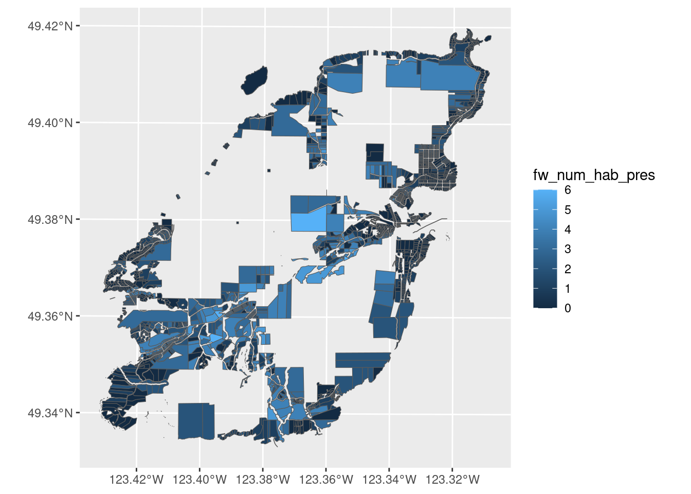
#### Convert to sf for better data.frame utilities ####
notprotected_cons_vals_sf <- notprotected_cons_3 %>%
  st_as_sf() %>%
  tidyr::replace_na(list( # Replace NAs with 0 in freshwater columns
    riparian = 0, 
    streams = 0, 
    lakes = 0, 
    ponds = 0, 
    wetlands = 0
  )) %>% 
  mutate(fw_num_hab_pres = rowSums(across(names(fw_rast_stack)), na.rm = T)) # Get number of habitat types in each parcel


#### PLOTTING ####
# Quick plot to check
ggplot(notprotected_cons_vals_sf) +
  geom_sf(aes(fill = fw_num_hab_pres))

# Caption for all maps
caption <- paste0("Map created: ", date(), ". Palen Lab. Created by Jay Matsushiba (jmatsush@sfu.ca)")

# Conservation Vals Continuous
conservation_vals_cont_gg <- function() {
  notprotected_public_colour <-  "green"
  notprotected_private_colour <- "red"
  list(
    geom_sf(data = notprotected_cons_vals_sf, aes(fill = rankmap), color = NA),
    scale_fill_viridis_c(),
    geom_sf(data = notprotected_privatelands, aes(colour = notprotected_private_colour), linewidth = 0.3, fill = NA),
    geom_sf(data = notprotected_publiclands, aes(colour = notprotected_public_colour), linewidth = 0.3, fill = NA),
    scale_colour_identity(
      name = "",
      breaks = c(notprotected_public_colour, notprotected_private_colour),
      labels = c("Unprotected Public", "Unprotected Private"),
      guide = "legend"
    ),
    ggnewscale::new_scale_fill(),
    ggnewscale::new_scale_colour()
  )
}
conservation_vals_cont_ggplot <- bowen_map_ggplot(
  conservation_vals_cont_gg,
  title = "Conservation Values by Unprotected Parcels",
  subtitle = "Mapping the unprotected parcels and their relative biodiversity values to identify potential parcels for future protection.",
  caption = caption
)

Reading layer `bowen_island_shoreline_w_hutt__bowen_islands' from data source 
  `/home/jay/Programming_Projects/bowen.biodiversity.webapp/data-raw/bowen_island_shoreline_w_hutt.gpkg' 
  using driver `GPKG'
Simple feature collection with 11 features and 1 field
Geometry type: POLYGON
Dimension:     XY
Bounding box:  xmin: 4001956 ymin: 2020764 xmax: 4013988 ymax: 2028901
Projected CRS: NAD83 / Statistics Canada Lambert
Loading basemap 'backdrop' from map service 'maptiler'...

<SpatRaster> resampled to 501000 cells.

ggplot2::ggsave(
  here(output_dir, "/", paste0(Sys.Date(), "_conservation_vals_continuous_parcels.png")),
  conservation_vals_cont_ggplot,
  device = ragg::agg_png,
  width = 9, height = 12, units = "in", res = 300
)

# Conservation Vals Top 30
conservation_vals_top_gg <- function() {
  notprotected_public_colour <-  "green"
  notprotected_private_colour <- "red"
  list(
    geom_sf(data = notprotected_cons_vals_sf, aes(fill = rankmap_top_30), color = NA),
    scale_fill_viridis_c(),
    geom_sf(data = notprotected_privatelands, aes(colour = notprotected_private_colour), linewidth = 0.3, fill = NA),
    geom_sf(data = notprotected_publiclands, aes(colour = notprotected_public_colour), linewidth = 0.3, fill = NA),
    scale_colour_identity(
      name = "",
      breaks = c(notprotected_public_colour, notprotected_private_colour),
      labels = c("Unprotected Public", "Unprotected Private"),
      guide = "legend"
    ),
    ggnewscale::new_scale_fill(),
    ggnewscale::new_scale_colour()
  )
}
conservation_vals_top_ggplot <- bowen_map_ggplot(
  conservation_vals_top_gg,
  title = "Top Conservation Values by Unprotected Parcels",
  subtitle = "Mapping the unprotected parcels and number of top 30% conservation value cells to identify potential parcels for future protection.",
  caption = caption
)

Reading layer `bowen_island_shoreline_w_hutt__bowen_islands' from data source 
  `/home/jay/Programming_Projects/bowen.biodiversity.webapp/data-raw/bowen_island_shoreline_w_hutt.gpkg' 
  using driver `GPKG'
Simple feature collection with 11 features and 1 field
Geometry type: POLYGON
Dimension:     XY
Bounding box:  xmin: 4001956 ymin: 2020764 xmax: 4013988 ymax: 2028901
Projected CRS: NAD83 / Statistics Canada Lambert
Loading basemap 'backdrop' from map service 'maptiler'...

<SpatRaster> resampled to 501000 cells.

ggplot2::ggsave(
  here(output_dir, "/", paste0(Sys.Date(), "_conservation_vals_top_parcels.png")),
  conservation_vals_top_ggplot,
  device = ragg::agg_png,
  width = 9, height = 12, units = "in", res = 300
)

# Freshwater sum richness
freshwater_sum_gg <- function() {
  notprotected_public_colour <-  "green"
  notprotected_private_colour <- "red"
  list(
    geom_sf(data = notprotected_cons_vals_sf, aes(fill = fw_sum_richness), color = NA),
    scale_fill_viridis_c(),
    geom_sf(data = notprotected_privatelands, aes(colour = notprotected_private_colour), linewidth = 0.3, fill = NA),
    geom_sf(data = notprotected_publiclands, aes(colour = notprotected_public_colour), linewidth = 0.3, fill = NA),
    scale_colour_identity(
      name = "",
      breaks = c(notprotected_public_colour, notprotected_private_colour),
      labels = c("Unprotected Public", "Unprotected Private"),
      guide = "legend"
    ),
    ggnewscale::new_scale_fill(),
    ggnewscale::new_scale_colour()
  )
}
freshwater_sum_ggplot <- bowen_map_ggplot(
  freshwater_sum_gg,
  title = "Relative Freshwater Habitat Richness by Unprotected Parcels",
  subtitle = "Mapping the unprotected parcels and the total sum of freshwater habitat richness cells to identify potential parcels for future protection.",
  caption = caption
)

Reading layer `bowen_island_shoreline_w_hutt__bowen_islands' from data source 
  `/home/jay/Programming_Projects/bowen.biodiversity.webapp/data-raw/bowen_island_shoreline_w_hutt.gpkg' 
  using driver `GPKG'
Simple feature collection with 11 features and 1 field
Geometry type: POLYGON
Dimension:     XY
Bounding box:  xmin: 4001956 ymin: 2020764 xmax: 4013988 ymax: 2028901
Projected CRS: NAD83 / Statistics Canada Lambert
Loading basemap 'backdrop' from map service 'maptiler'...

<SpatRaster> resampled to 501000 cells.

ggplot2::ggsave(
  here(output_dir, "/", paste0(Sys.Date(), "_fw_sum_richness_parcels.png")),
  freshwater_sum_ggplot,
  device = ragg::agg_png,
  width = 9, height = 12, units = "in", res = 300
)
# Freshwater num habitats richness
freshwater_num_hab_gg <- function() {
  notprotected_public_colour <-  "green"
  notprotected_private_colour <- "red"
  list(
    geom_sf(data = notprotected_cons_vals_sf, aes(fill = fw_num_hab_pres), color = NA),
    scale_fill_viridis_c(),
    geom_sf(data = notprotected_privatelands, aes(colour = notprotected_private_colour), linewidth = 0.3, fill = NA),
    geom_sf(data = notprotected_publiclands, aes(colour = notprotected_public_colour), linewidth = 0.3, fill = NA),
    scale_colour_identity(
      name = "",
      breaks = c(notprotected_public_colour, notprotected_private_colour),
      labels = c("Unprotected Public", "Unprotected Private"),
      guide = "legend"
    ),
    ggnewscale::new_scale_fill(),
    ggnewscale::new_scale_colour()
  )
}
freshwater_num_hab_ggplot <- bowen_map_ggplot(
  freshwater_num_hab_gg,
  title = "Number of Freshwater Habitats in Unprotected Parcels",
  subtitle = "Mapping the unprotected parcels and number of freshwater habitat types present to identify potential parcels for future protection.",
  caption = caption
)

Reading layer `bowen_island_shoreline_w_hutt__bowen_islands' from data source 
  `/home/jay/Programming_Projects/bowen.biodiversity.webapp/data-raw/bowen_island_shoreline_w_hutt.gpkg' 
  using driver `GPKG'
Simple feature collection with 11 features and 1 field
Geometry type: POLYGON
Dimension:     XY
Bounding box:  xmin: 4001956 ymin: 2020764 xmax: 4013988 ymax: 2028901
Projected CRS: NAD83 / Statistics Canada Lambert
Loading basemap 'backdrop' from map service 'maptiler'...

<SpatRaster> resampled to 501000 cells.

ggplot2::ggsave(
  here(output_dir, "/", paste0(Sys.Date(), "_fw_num_hab_parcels.png")),
  freshwater_num_hab_ggplot,
  device = ragg::agg_png,
  width = 9, height = 12, units = "in", res = 300
)

#### PLOTTING PUBLIC LANDS ####
# Conservation Vals Continuous
conservation_vals_cont_pub_gg <- function() {
  list(
    geom_sf(data = notprotected_cons_vals_sf[!notprotected_cons_vals_sf$OwnerType %in% c("Private", "Mixed Ownership", "Unclassified"),] , aes(fill = rankmap), color = NA),
    scale_fill_viridis_c(),
    ggnewscale::new_scale_fill(),
    ggnewscale::new_scale_colour()
  )
}
conservation_vals_cont_pub_ggplot <- bowen_map_ggplot(
  conservation_vals_cont_pub_gg,
  title = "Conservation Values by Unprotected Parcels",
  subtitle = "Mapping the unprotected parcels and their relative biodiversity values to identify potential parcels for future protection.",
  caption = caption
)

Reading layer `bowen_island_shoreline_w_hutt__bowen_islands' from data source 
  `/home/jay/Programming_Projects/bowen.biodiversity.webapp/data-raw/bowen_island_shoreline_w_hutt.gpkg' 
  using driver `GPKG'
Simple feature collection with 11 features and 1 field
Geometry type: POLYGON
Dimension:     XY
Bounding box:  xmin: 4001956 ymin: 2020764 xmax: 4013988 ymax: 2028901
Projected CRS: NAD83 / Statistics Canada Lambert
Loading basemap 'backdrop' from map service 'maptiler'...

<SpatRaster> resampled to 501000 cells.

ggplot2::ggsave(
  here(output_dir, "/", paste0(Sys.Date(), "_conservation_vals_continuous_pub_parcels.png")),
  conservation_vals_cont_pub_ggplot,
  device = ragg::agg_png,
  width = 9, height = 12, units = "in", res = 300
)

# Conservation Vals Top 30
conservation_vals_top_pub_gg <- function() {
  list(
    geom_sf(data = notprotected_cons_vals_sf[!notprotected_cons_vals_sf$OwnerType %in% c("Private", "Mixed Ownership", "Unclassified"),], aes(fill = rankmap_top_30), color = NA),
    scale_fill_viridis_c(),
    ggnewscale::new_scale_fill(),
    ggnewscale::new_scale_colour()
  )
}
conservation_vals_top_pub_ggplot <- bowen_map_ggplot(
  conservation_vals_top_pub_gg,
  title = "Top Conservation Values by Unprotected Parcels",
  subtitle = "Mapping the unprotected parcels and number of top 30% conservation value cells to identify potential parcels for future protection.",
  caption = caption
)

Reading layer `bowen_island_shoreline_w_hutt__bowen_islands' from data source 
  `/home/jay/Programming_Projects/bowen.biodiversity.webapp/data-raw/bowen_island_shoreline_w_hutt.gpkg' 
  using driver `GPKG'
Simple feature collection with 11 features and 1 field
Geometry type: POLYGON
Dimension:     XY
Bounding box:  xmin: 4001956 ymin: 2020764 xmax: 4013988 ymax: 2028901
Projected CRS: NAD83 / Statistics Canada Lambert
Loading basemap 'backdrop' from map service 'maptiler'...

<SpatRaster> resampled to 501000 cells.

ggplot2::ggsave(
  here(output_dir, "/", paste0(Sys.Date(), "_conservation_vals_top_pub_parcels.png")),
  conservation_vals_top_pub_ggplot,
  device = ragg::agg_png,
  width = 9, height = 12, units = "in", res = 300
)

# Freshwater sum richness
freshwater_sum_pub_gg <- function() {
  list(
    geom_sf(data = notprotected_cons_vals_sf[!notprotected_cons_vals_sf$OwnerType %in% c("Private", "Mixed Ownership", "Unclassified"),], aes(fill = fw_sum_richness), color = NA),
    scale_fill_viridis_c(),
    ggnewscale::new_scale_fill(),
    ggnewscale::new_scale_colour()
  )
}
freshwater_sum_pub_ggplot <- bowen_map_ggplot(
  freshwater_sum_pub_gg,
  title = "Relative Freshwater Habitat Richness by Unprotected Parcels",
  subtitle = "Mapping the unprotected parcels and the total sum of freshwater habitat richness cells to identify potential parcels for future protection.",
  caption = caption
)

Reading layer `bowen_island_shoreline_w_hutt__bowen_islands' from data source 
  `/home/jay/Programming_Projects/bowen.biodiversity.webapp/data-raw/bowen_island_shoreline_w_hutt.gpkg' 
  using driver `GPKG'
Simple feature collection with 11 features and 1 field
Geometry type: POLYGON
Dimension:     XY
Bounding box:  xmin: 4001956 ymin: 2020764 xmax: 4013988 ymax: 2028901
Projected CRS: NAD83 / Statistics Canada Lambert
Loading basemap 'backdrop' from map service 'maptiler'...

<SpatRaster> resampled to 501000 cells.

ggplot2::ggsave(
  here(output_dir, "/", paste0(Sys.Date(), "_fw_sum_richness_pub_parcels.png")),
  freshwater_sum_pub_ggplot,
  device = ragg::agg_png,
  width = 9, height = 12, units = "in", res = 300
)
# Freshwater num habitats richness
freshwater_num_hab_pub_gg <- function() {
  list(
    geom_sf(data = notprotected_cons_vals_sf[!notprotected_cons_vals_sf$OwnerType %in% c("Private", "Mixed Ownership", "Unclassified"),], aes(fill = fw_num_hab_pres), color = NA),
    scale_fill_viridis_c(),
    ggnewscale::new_scale_fill(),
    ggnewscale::new_scale_colour()
  )
}
freshwater_num_hab_pub_ggplot <- bowen_map_ggplot(
  freshwater_num_hab_pub_gg,
  title = "Number of Freshwater Habitats in Unprotected Parcels",
  subtitle = "Mapping the unprotected parcels and number of freshwater habitat types present to identify potential parcels for future protection.",
  caption = caption
)

Reading layer `bowen_island_shoreline_w_hutt__bowen_islands' from data source 
  `/home/jay/Programming_Projects/bowen.biodiversity.webapp/data-raw/bowen_island_shoreline_w_hutt.gpkg' 
  using driver `GPKG'
Simple feature collection with 11 features and 1 field
Geometry type: POLYGON
Dimension:     XY
Bounding box:  xmin: 4001956 ymin: 2020764 xmax: 4013988 ymax: 2028901
Projected CRS: NAD83 / Statistics Canada Lambert
Loading basemap 'backdrop' from map service 'maptiler'...

<SpatRaster> resampled to 501000 cells.

ggplot2::ggsave(
  here(output_dir, "/", paste0(Sys.Date(), "_fw_num_hab_pub_parcels.png")),
  freshwater_num_hab_pub_ggplot,
  device = ragg::agg_png,
  width = 9, height = 12, units = "in", res = 300
)

Crown Land - Outside of Parcels

Polygon extent of unprotected crown land not in parcels

# Dissolve protected areas into one geometry
dissolved_protectedareas <- bowen_protectedareas_valid %>%
  summarise() %>%
  st_cast() %>%
  st_buffer(1) 

crown_valid <- crown %>% 
  st_snap(x = ., y = ., tolerance = 0.1) %>%
  st_make_valid() 
notprotected_crown <- st_difference(crown_valid, dissolved_protectedareas)

Warning: attribute variables are assumed to be spatially constant throughout
all geometries

# Manually check each crown land polygon
for(i in 1:nrow(notprotected_crown)) {
  plot(notprotected_crown[i,])
}

# Remove polygons that should not be included in notprotected areas 
# rowname 1 (Fairy Fen Natural Reserve), sliver
# rowname 74 (Seymour Bay Park), wrong polygon in the first place
notprotected_crown_clean <- notprotected_crown[!rownames(notprotected_crown) %in% c("1","74"),]

Identify potential protected areas within crown land not in parcels

Rasterize layer Identify candidate protected areas Two ways that crown land can be good candidates 1. High value pixels that are contiguous with other protected areas Things that fall under the top 30% are adjacent to protected areas Ex. large areas west of Killarney Lake, northeast corner of Bowen Island,

Contiguous pixels of high value that are not connected to protected areas Large enough for arguing for protection, 10 to 50 hectares or bigger

Great place to start using prioritizr! https://prioritizr.net/

Inputs

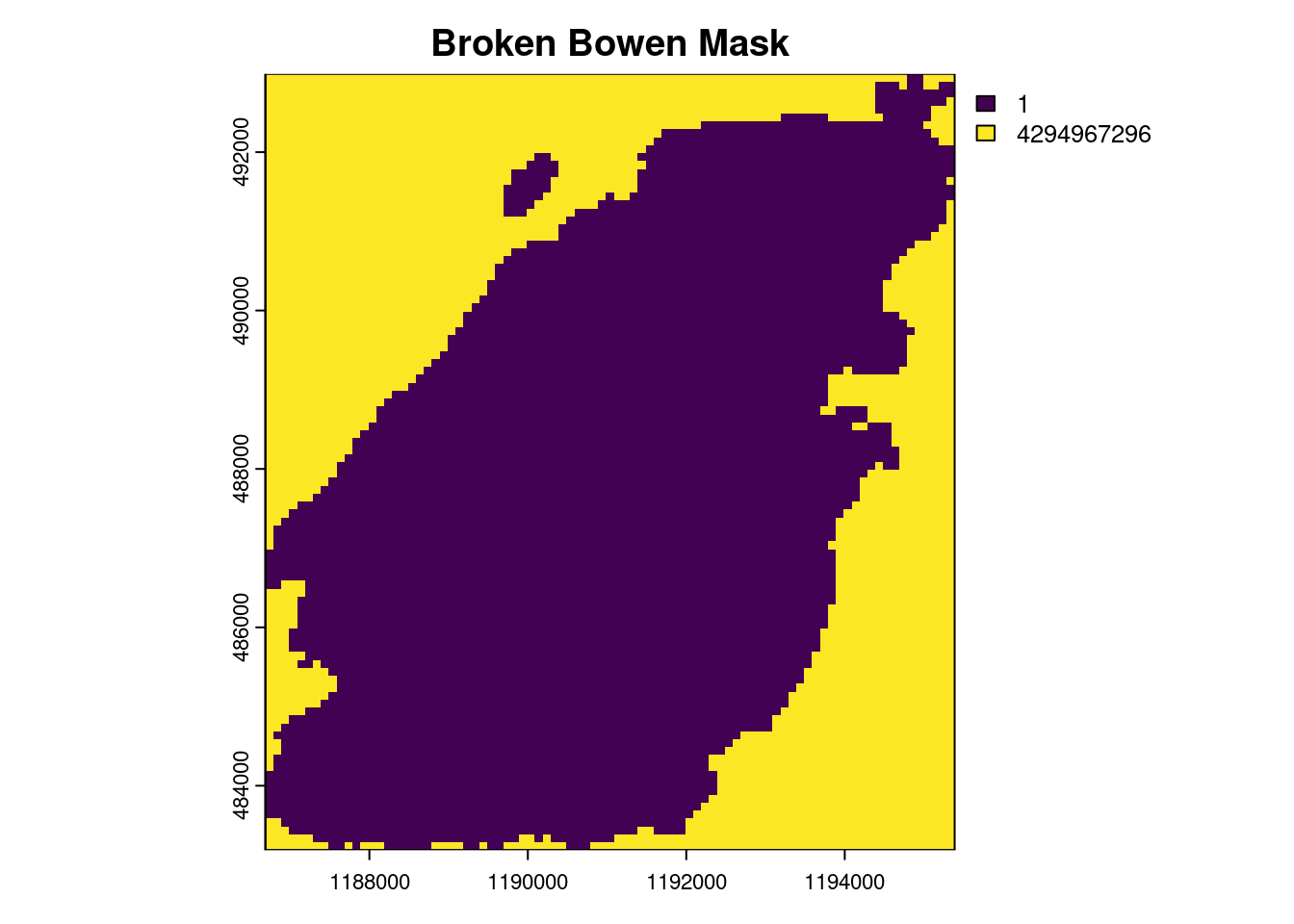
bowen_mask_broken <- rast(here("inst/extdata/bowen_mask.tif")) %>%
  project(zonation)
# for some reason, when bowen_mask is reprojected to match the zonation
# raster, it ends up changing NA values to an extremely large number. 
# probably some bit rollover issue?
plot(bowen_mask_broken, main = "Broken Bowen Mask")

bowen_mask_broken %>%
  values() %>%
  max() # 4294967296

[1] 4294967296

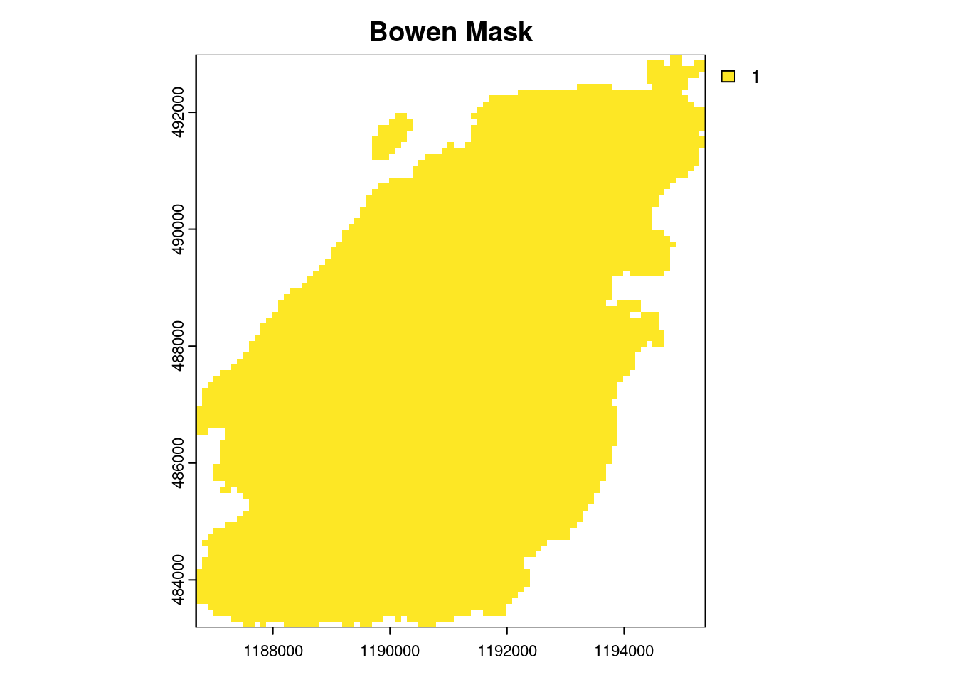
# this value is the highest unsigned 32-bit integer
# https://github.com/rspatial/terra/issues/1356
# seems like this issue has been reported, but not fixed

# planning units
bowen_mask <- rast(here("inst/extdata/bowen_mask.tif")) %>%
  project(zonation) %>% 
  mask(zonation) 

plot(bowen_mask, main = "Bowen Mask")

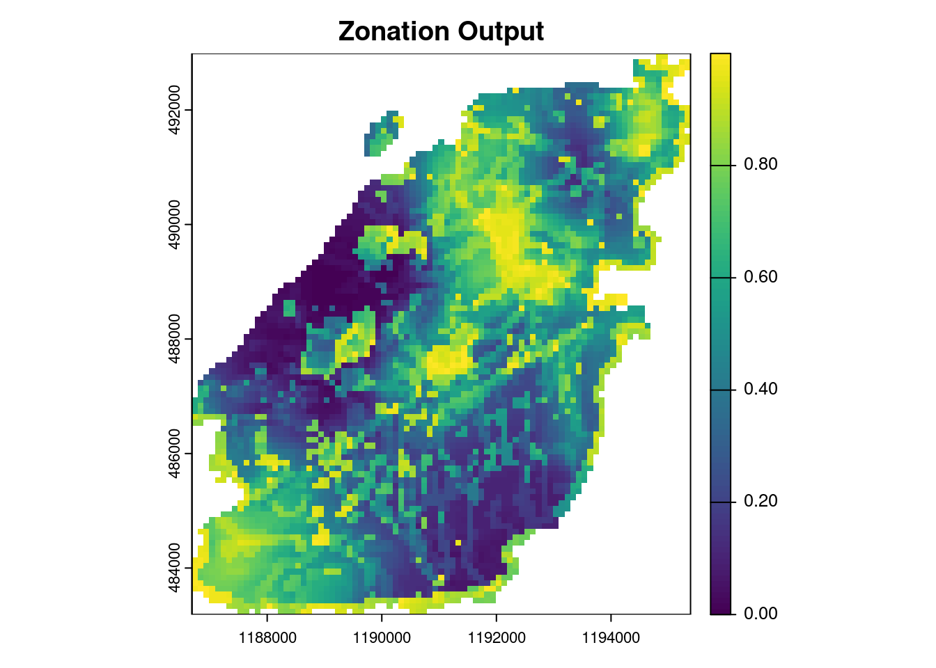
# features
plot(zonation, main = "Zonation Output")

Prioritizr

# calculate budget, get prop of pixels of planning units
prop_pixels <- 0.3 # for some reason, this provides weird results when not large enough
budget <- terra::global(bowen_mask, "sum", na.rm = T)[[1]] * prop_pixels 

# create problem
p1 <- problem(bowen_mask, features = zonation) %>%
  add_min_shortfall_objective(budget) %>%
  add_relative_targets(1) %>% # need to be at least double the budget
  # since we only have one feature, this target is meaningless but is a
  # requirement for priortizr to work 
  add_binary_decisions() %>%
  add_default_solver(gap = 0.05, verbose = FALSE) 
  # gap needs to be smaller than the difference between prop_pixels and locked constraints
  # if this is not, leads to nonsensical solutions 
  # gap value is the % from optimal
  # therefore, if gap is too large, then any solution is close enough to optimal

# print conservation problem
print(p1)

A conservation problem (<ConservationProblem>)
├•data
│├•features:    "rankmap"
│└•planning units:
│ ├•data:       <SpatRaster> (5314 total)
│ ├•costs:      constant values (all equal to 1)
│ ├•extent:     1186687.5, 483187.5, 1195387.5, 492987.5 (xmin, ymin, xmax, ymax)
│ └•CRS:        NAD83 / BC Albers (projected)
├•formulation
│├•objective:   minimum shortfall objective (`budget` = 1594.2)
│├•penalties:   none specified
│├•targets:     relative targets (between 1 and 1)
│├•constraints: none specified
│└•decisions:   binary decision
└•optimization
 ├•portfolio:   default portfolio
 └•solver:      gurobi solver (`gap` = 0.05, `time_limit` = 2147483647, `first_feasible` = FALSE, …)
# ℹ Use `summary(...)` to see complete formulation.

presolve_check(p1)

Warning in presolve_check(compile(x), warn = warn): Problem failed presolve checks.

These checks indicate that solutions might not identify meaningful priority
areas:

✖ The problem only contains a single feature.
→ Conservation planning generally requires multiple features (e.g., species,
  ecosystem types) to identify meaningful priority areas.

ℹ For more information, see `presolve_check()`.

[1] FALSE

s1 <- solve(p1, force = T)

Warning in solve(p1, force = T): → Problem failed presolve checks.

These checks indicate that solutions might not identify meaningful priority
areas:

✖ The problem only contains a single feature.
→ Conservation planning generally requires multiple features (e.g., species,
  ecosystem types) to identify meaningful priority areas.

ℹ For more information, see `presolve_check()`.

# extract the objective
print(attr(s1, "objective"))

solution_1 
 0.4900132

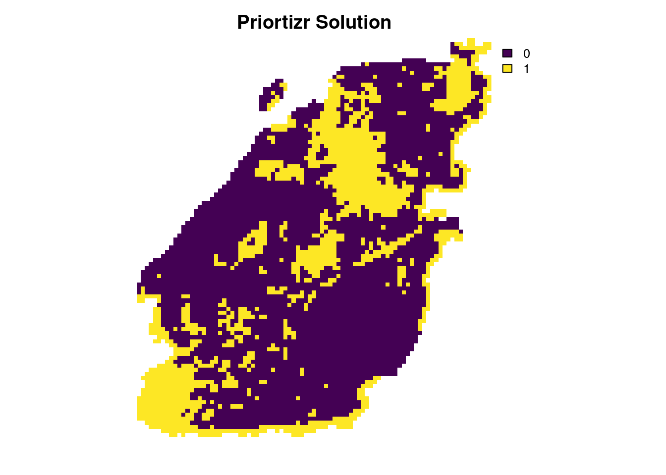
# compare plots, check for agreement between priortizr and zonation
plot(s1, main = "Priortizr Solution", axes = FALSE)

remove_by_quantile(zonation, 1 - prop_pixels) %>%
  plot(main = "Top Zonation Pixels")

# check for number of cells 
s1 %>% values() %>% sum(na.rm = T) # 265 cells selected

[1] 1594

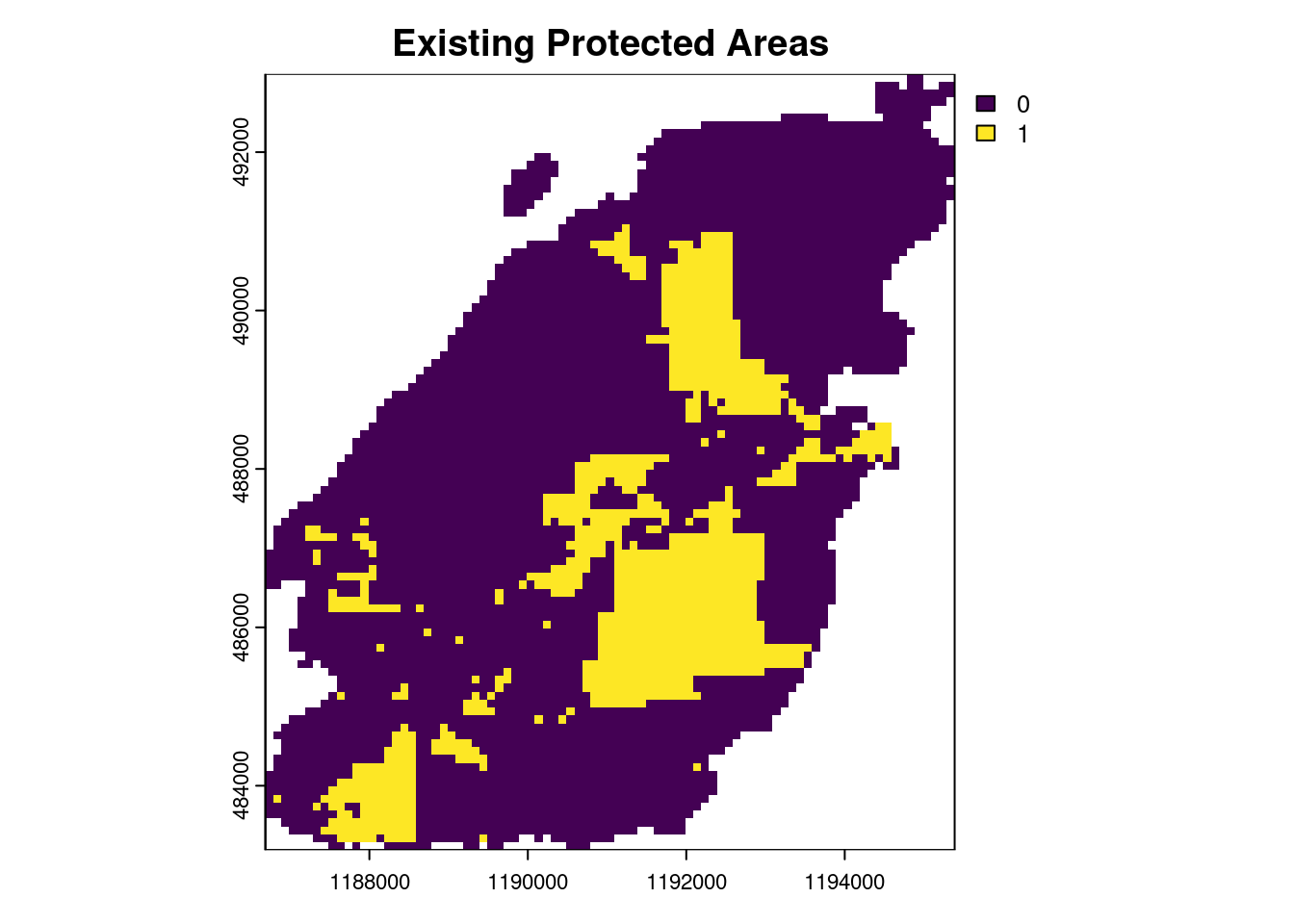
# it works! basic top pixels identified, and agrees with zonation
# the main goal is to not use priortizr for conservation values
# the goal is to use the constraints and penalties that are part 
# of the package

# Existing Protected Areas
bowen_protectedareas %>% plot()

# trying removing covenants, since very fragmented
bowen_pa_rast <- bowen_protectedareas[bowen_protectedareas$type != "Covenants",] %>%
  vect() %>%
  project(bowen_mask) %>%
  rasterize(bowen_mask, background = 0) %>%
  mask(bowen_mask) 

# bowen_pa_rast_2 <- bowen_protectedareas %>%
#   vect() %>%
#   project(bowen_mask) %>%
#   rasterize(bowen_mask, background = 0) %>%
#   mask(bowen_mask) 

bowen_pa_cell_count <- bowen_pa_rast %>%
  values() %>%
  sum(na.rm = T)
bowen_pa_prop <- bowen_pa_cell_count / sum(values(bowen_mask), na.rm = T)

plot(bowen_pa_rast, main = "Existing Protected Areas")

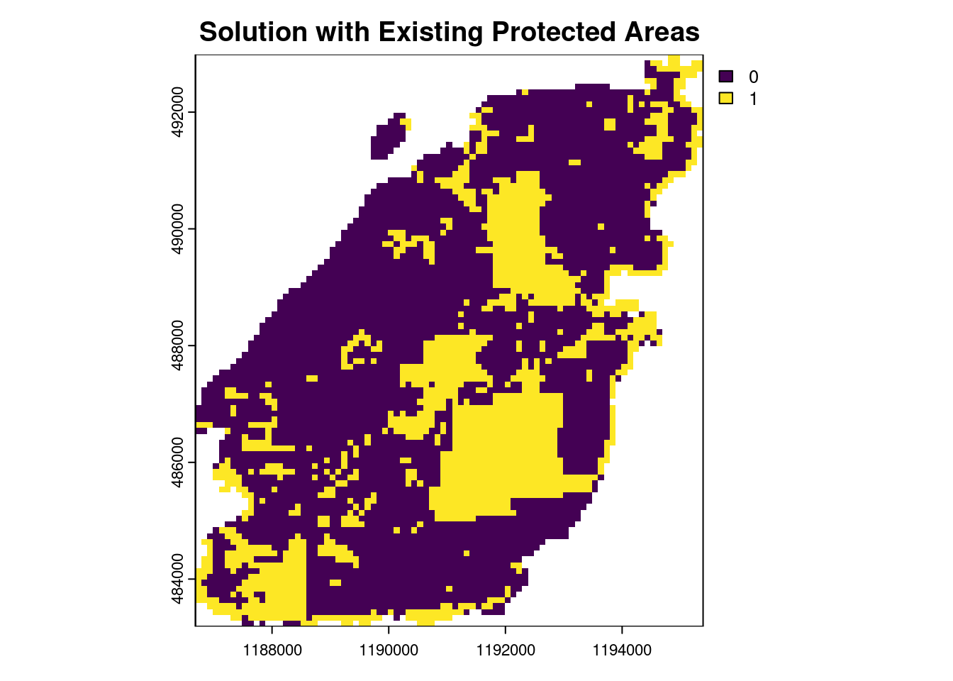
# create new problem with locked in constraints 
p2 <- 
  p1 %>%
  add_locked_in_constraints(bowen_pa_rast)

s2 <- solve(p2, force = T)

Warning in solve(p2, force = T): → Problem failed presolve checks.

These checks indicate that solutions might not identify meaningful priority
areas:

✖ The problem only contains a single feature.
→ Conservation planning generally requires multiple features (e.g., species,
  ecosystem types) to identify meaningful priority areas.

ℹ For more information, see `presolve_check()`.

plot(s2, main = "Solution with Existing Protected Areas")

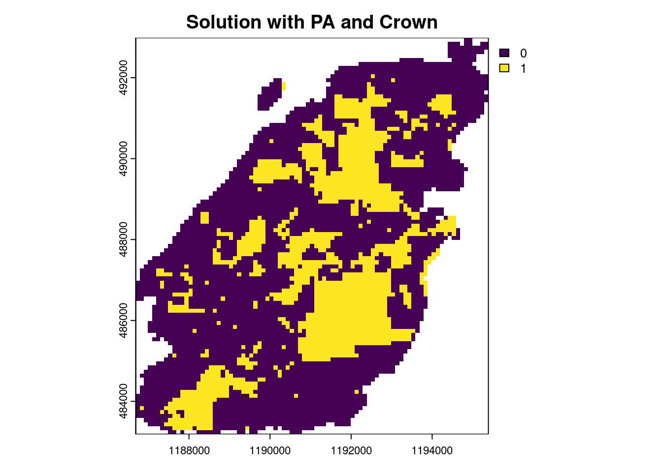
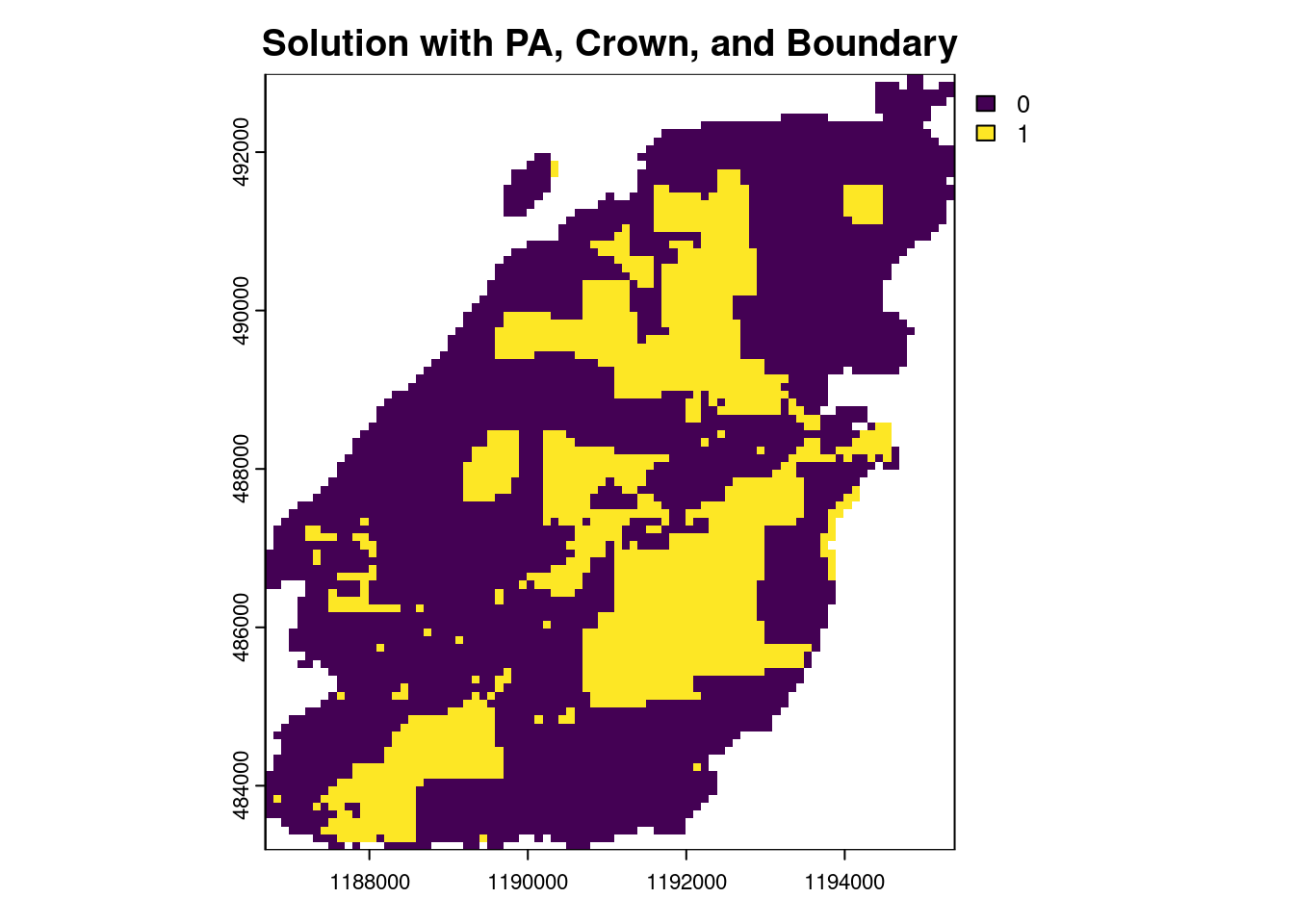
# Crown land
## Maybe combine analysis with parcels? 
## Keep seperate for now, combine later

crown_rast <- crown %>%
  vect() %>%
  project(bowen_mask) %>%
  rasterize(bowen_mask, background = 0, touches = T) %>%
  mask(bowen_mask)

# need to make sure it includes the protected areas
crown_pa <- max(c(crown_rast, bowen_pa_rast))

# reverse for locked out constraints
m <- rbind(
  c(0, 1),
  c(1, 0)
)

lockedout <- crown_pa %>%
  classify(m)

# create new problem with locked out constraints
p3 <-
  p2 %>%
  add_locked_out_constraints(lockedout)
s3 <- solve(p3, force = T)

Warning in solve(p3, force = T): → Problem failed presolve checks.

These checks indicate that solutions might not identify meaningful priority
areas:

✖ The problem only contains a single feature.
→ Conservation planning generally requires multiple features (e.g., species,
  ecosystem types) to identify meaningful priority areas.

ℹ For more information, see `presolve_check()`.

plot(s3, main = "Solution with PA and Crown")

# add boundary penalties
p4 <-
  p3 %>%
  add_boundary_penalties(penalty = 0.000001, edge_factor = 0.5)
s4 <- solve(p4, force = T)

Warning in solve(p4, force = T): → Problem failed presolve checks.

These checks indicate that solutions might not identify meaningful priority
areas:

✖ The problem only contains a single feature.
→ Conservation planning generally requires multiple features (e.g., species,
  ecosystem types) to identify meaningful priority areas.

ℹ For more information, see `presolve_check()`.

s4 %>% values() %>% sum(na.rm = T) # 1593

[1] 1586

# the total pixels selected under no boundary penalty is 1594
# therefore, with this penalty value of 0.000001
# boundary penalty has an effect, but not overly so that 
# step just selects pixels around existing protected areas

plot(s4, main = "Solution with PA, Crown, and Boundary")

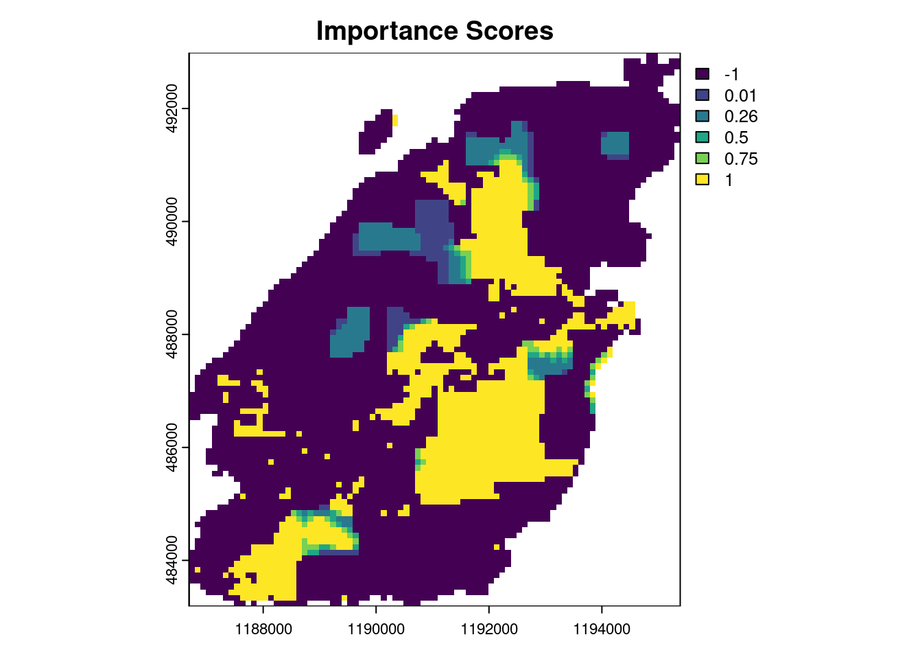
# importance scores
imp <- 
  p4 %>%
  eval_rank_importance(s4, n = 5, force = T)

Warning in matrix(compile(x)$lb(), ncol = n_z, nrow = n_pu): data length
[15687] is not a sub-multiple or multiple of the number of rows [5314]

Warning in .local(x, solution, ...): → Problem failed presolve checks.

These checks indicate that solutions might not identify meaningful priority
areas:

✖ The problem only contains a single feature.
→ Conservation planning generally requires multiple features (e.g., species,
  ecosystem types) to identify meaningful priority areas.

ℹ For more information, see `presolve_check()`.

print(imp)

class       : SpatRaster 
dimensions  : 98, 87, 1  (nrow, ncol, nlyr)
resolution  : 100, 100  (x, y)
extent      : 1186688, 1195388, 483187.5, 492987.5  (xmin, xmax, ymin, ymax)
coord. ref. : NAD83 / BC Albers (EPSG:3005) 
source(s)   : memory
varname     : rankmap 
name        : rs 
min value   :  0 
max value   :  1

imp <- terra::mask(imp, s4, maskvalues = 0, updatevalue = -1)
plot(imp, main = "Importance Scores")

# remove existing protected areas 
m <- c(
  -1, 0, NA
)
imp_clean <- (imp - 2 * bowen_pa_rast) %>%
  ifel(. <= -1, NA, .)

Plotting

# gg
crown_poten_ggfunc <- function() {
  protected_colour <- "#b3e2cd"
  parcels_colour <-  "#fdcdac"
  output <- list(
    geom_spatraster(data = imp_clean, na.rm = T),
    scale_fill_viridis_c(na.value = NA, name = "Protected Area Potential"),
    ggnewscale::new_scale_fill(),
    geom_sf(data = parcels, aes(fill = parcels_colour)),
    geom_sf(data = bowen_protectedareas_valid, aes(fill = protected_colour)),
    scale_fill_identity(name = "",
                          breaks = c(protected_colour, parcels_colour),
                          labels = c("Protected", "Parcels"),
                          guide = "legend"
    ),
    ggnewscale::new_scale_fill(),
    ggnewscale::new_scale_colour()
  )
  return(output)
}
crown_poten_ggplot <- bowen_map_ggplot(
  crown_poten_ggfunc,
  title = "Top Locations for Protected Areas (30x30)",
  subtitle = "Mapping optimal Crown land for reaching 30x30 targets, using the conservation values analysis and existing protected areas. This output considers connectivity by applying boundary penalties, which prioritizes shorter boundaries relative to area. Currently, about 20% of Bowen Island is under some protection.",
  caption = caption
)

Reading layer `bowen_island_shoreline_w_hutt__bowen_islands' from data source 
  `/home/jay/Programming_Projects/bowen.biodiversity.webapp/data-raw/bowen_island_shoreline_w_hutt.gpkg' 
  using driver `GPKG'
Simple feature collection with 11 features and 1 field
Geometry type: POLYGON
Dimension:     XY
Bounding box:  xmin: 4001956 ymin: 2020764 xmax: 4013988 ymax: 2028901
Projected CRS: NAD83 / Statistics Canada Lambert
Loading basemap 'backdrop' from map service 'maptiler'...

<SpatRaster> resampled to 501000 cells.

ggplot2::ggsave(
  here(output_dir, "/", paste0(Sys.Date(), "_crown_potential.png")),
  crown_poten_ggplot,
  device = ragg::agg_png,
  width = 9, height = 12, units = "in", res = 300
)