Threats: Fire

Author

Jay Matsushiba

Published

September 12, 2025

Code

# This repository, access to data objects created for this project 
library(bowen.biodiversity.webapp)

# Spatial data packages
library(sf)
library(terra)

# Visualization 
library(ggplot2)
library(leaflet)
library(tidyterra)

# Utilities 
library(here)
library(tidyverse)

Threats: Wildfire

One major potential threat for biodiversity on Bowen Island is wildfire. We wanted to analyze the spatial overlap between Conservation Values output we generated and wildfire impacts. With this, we could understand where on Bowen Island would be relatively more affected if/when a wildfire occurs.

Existing Data Sources

Rather than creating our own wildfire index, we first explored what datasets existed. This section describes the data that we are aware of, and their strengths and limitations.

Bowen Wildland Urban Interfaces (WUI)

Bowen Island WIldland Urban Interface Map

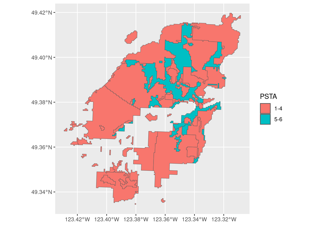
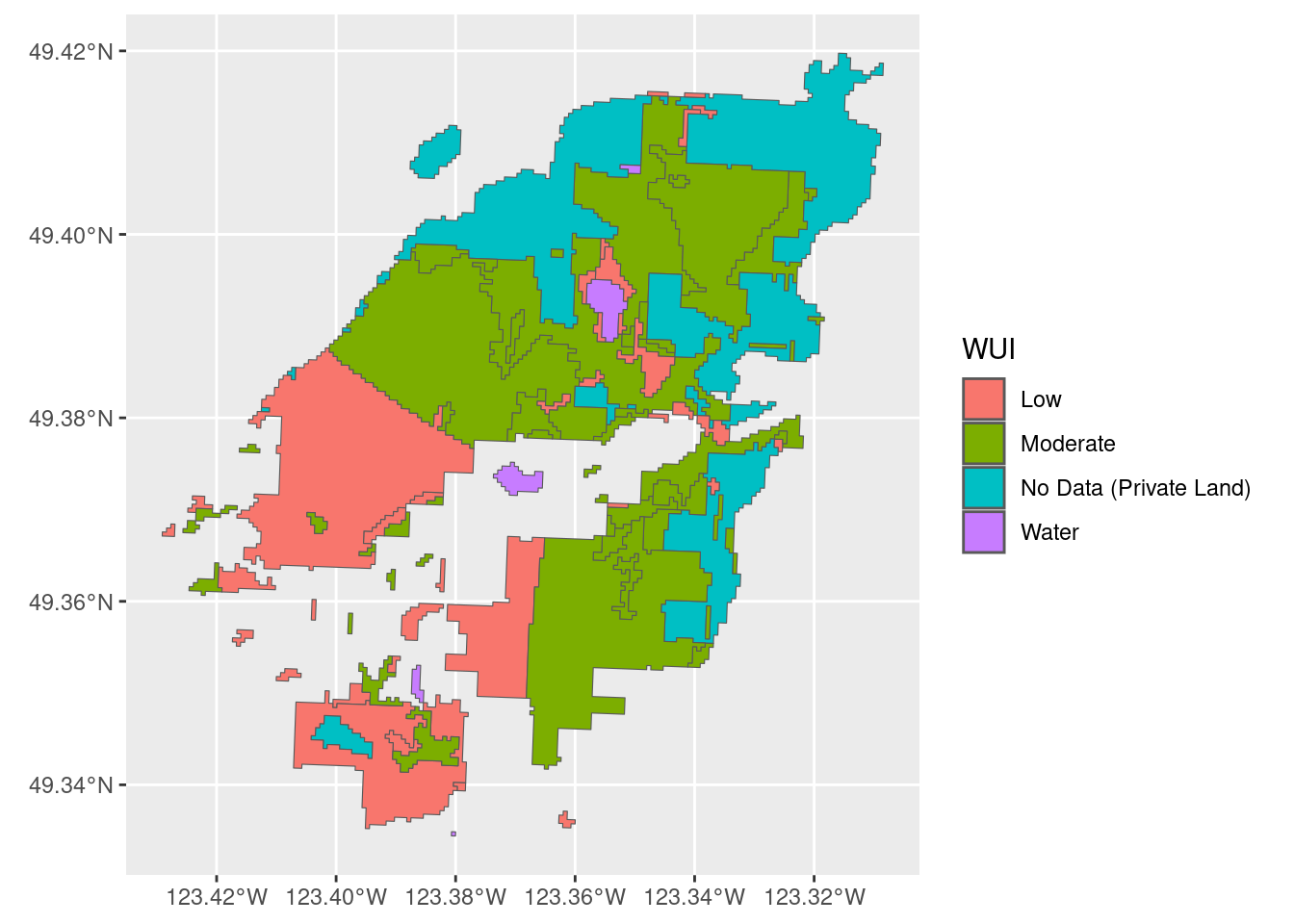
The Province of British Columbia produces the Wildland Urban Interface (WUI) maps, with their intention being to use these maps to inform the relative impact of wildfires on human development. These maps take into consideration three key variables - fuel load, climate conditons, and human development at the interface between urban and wildland areas. The intended use case for these maps are to inform wildfire prevention and response in British Columbia.

The WUI seems to be rigourous in their modelling of fuel load and climate conditions, but because these values are not provided separately from the final WUI map, we are not able to use these layers for our purposes. For our purposes, we want to look at how wildfires would impact biodiversity, and would need to remove the human development variable. Therefore, after exploring the data, we have elected not to use the WUI map to estimate the vulnerability of biodiversity to wildfires.

Sources: BC Wildfire Service: WUI

Preparing WUI Downloaded Layers

The original WUI maps are provided as a KMZ file. The KMZ files were first loaded into QGIS and clipped to data-raw/bowen_boundary/Bowen_boundary.shp. This clipped KMZ was saved as data-raw/bowen_wui.gpkg.

Code

bowen_wui <- here("data-raw/bowen_wui.gpkg") %>% 
  st_read(quiet = T) %>%
  select(Name, PSTA) %>%
  rename(WUI = Name) %>%
  mutate(WUI_PSTA = paste0(WUI, "_", PSTA))

ggplot(bowen_wui) + 
  geom_sf(aes(fill = PSTA))

Code

ggplot(bowen_wui) + 
  geom_sf(aes(fill = WUI))

Code

ggplot(bowen_wui) + 
  geom_sf(aes(fill = WUI_PSTA))

Rasterizing WUI Maps

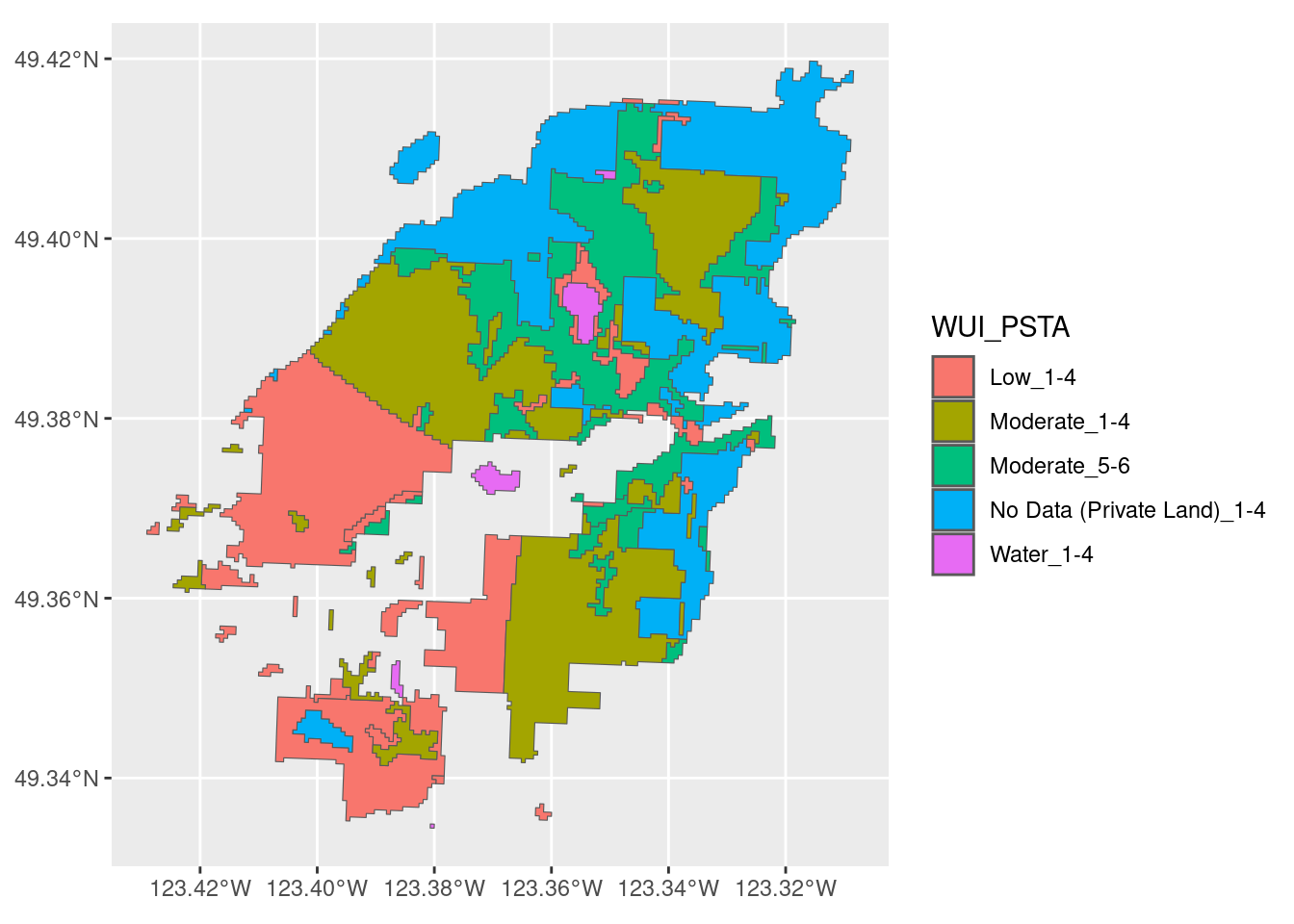
In case we would like to overlap the WUI risk classification with the Conservation Values raster, we need to rasterize the vector WUI layer.

[1] "Moderate_5-6"               "No Data (Private Land)_1-4"
[3] "Water_1-4"                  "Low_1-4"                   
[5] "Moderate_1-4"

Wildfire Vulnerability Index

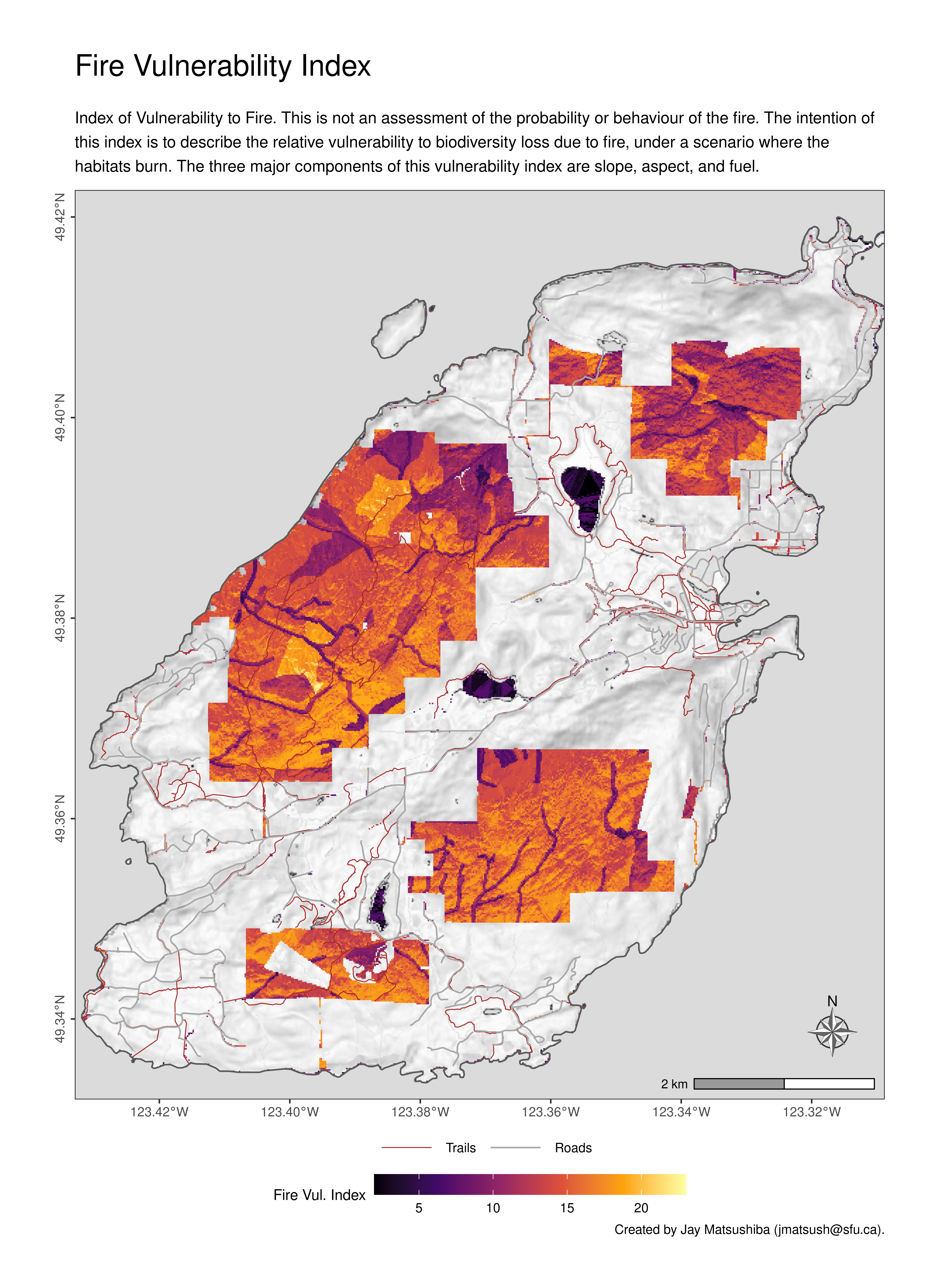
Since the existing data sources that we could identify do not suit our use case, we decided to create our own Wildfire Vulnerability Index. To clarify, this index does not assess the probability, severity, or behaviour of wildfire. Instead, we want to know the relative vulnerability to biodiversity loss due to fire, given a wildfire situation.

Three major components of vulnerability:

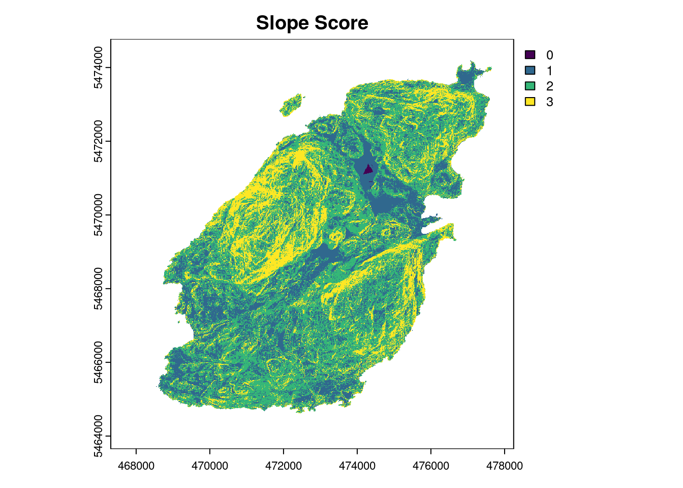
Slope. Fires spread more quickly when they move uphill. Relative ranking might look like this:

Slope Description	Score
0-10 degree slopes: lower vulnerability	1
10-30 degrees: moderate vulnerability	2
Above 30 degrees: higher vulnerability	3

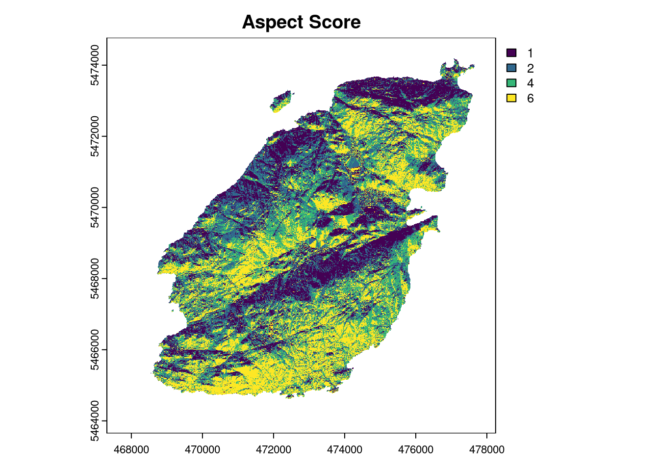
Aspect. Southerly exposures burn hotter, fire spreads more quickly, effects more uniform and destructive than on northern exposures, all else being equal. Might consider this as a first approximation:

Aspect Description	Score
0-45: Low vulnerability because fires unlikely to spread as fast or burn as hot	1
45-90: moderately low	2
90-135: moderately high	4
135-225: southerly exposures burn hotter, spread quickly and more uniformly	6
225-270: Moderately high	4
270-315 Moderately low	2
315-360: Low vulnerability	1

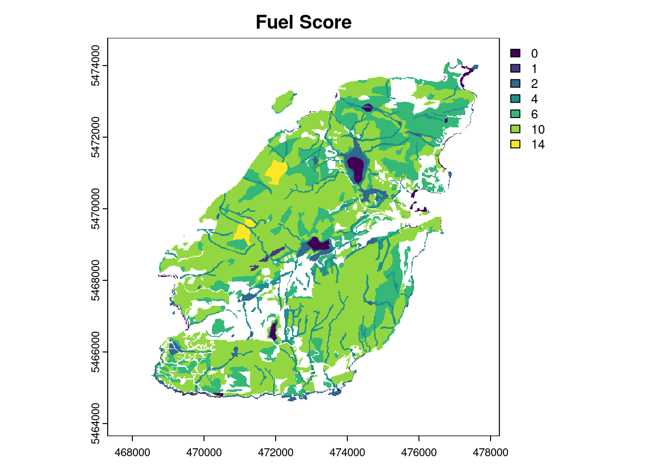
Fuels. On Bowen, the main differences in fuel loads have to do with whether a location is forested or not forested. Forested areas burn hotter and longer and long, hot burns have a more detrimental effect that shorter less intense fires. So the main distinctions should be made between forested and unforested. Forest stands comprised of larger trees are, of course, of higher value to biodiversity than denser stands with smaller trees, so we would like to be able to distinguish between forest structures to some degree. At the same time, when more mesic habitats burn the biodiversity effects tend to be high, because species are not adapted to fire. So we will need to rank habitats based on the differential effects of forest fuels present, as well as the difference in flora and fauna that make those locations more or less vulnerable in terms of biodiversity loss.

First Cut Ranking Scheme:

Habitat Description	Score
Forest, large/old trees	14
Forest, mature second growth	10
Forest, young regrowth	6
Shrublands	6
Grasslands: often burn and effects are modest, even positive in some cases	2
Riparian: seldom burns, but if it burns biodiversity effects may be very negative	4
Wetlands: seldom burn, more often they create fire breaks	2
Water: does not burn, but is vulnerable to ash deposition	0
Built environment (default to WUI map when talking about the built environment)	NA

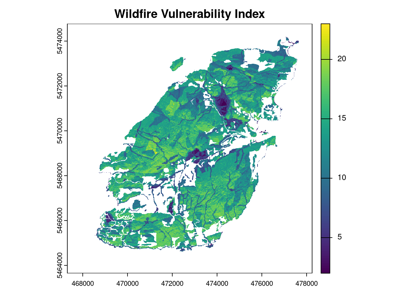
We conducted our further work around these basic ideas:

We pursue an index of vulnerability, rather than a more sophisticated approach to modeling fire or adapting an index that was developed for other purposes (i.e. WUI).
We create a simple index that allows us to compare the relative vulnerability of all locations on Bowen (with the exception of the built environment).
We consider slope, aspect, and fuels by habitat as the three components of an index.
We determine the relative ranks within each of the three components
Integrate the scores into an index that produces an aggregate vulnerability index score for each pixel. As a first approximation, this should be the additive (sum) of the three components – and then let’s see how that performs.

Generate Wildfire Vulnerability Index Raster

Input Data 1: LiDAR

We prepared the slope and aspect rasters from the LiDAR data provided by BC LiDAR. We then assigned the scores to these rasters according to the above scoring tables.

See Bowen Island DTM for more details.

Input Data 2: Metro Vancouver Sensitive Ecosystem Inventory (MVSEI)

The Metro Vancouver Sensitive Ecosystem Inventory (MVSEI) provides almost full coverage of habitat types across Bowen Island. The locations that do not have habitat type data from the MVSEI are those that have been subject to human development, and are no longer considered to be habitat. The more general classifications of the MVSEI make it easier to assign the scores, compared to using the Terrestrial Ecosystem Mapping (TEM) products.

Code

# Slope Score
## Create slope raster from LiDAR data
slope <- rast(here("data/bowen_slope.tif"))
## Create matrix of scores
### 1 0-10 degree slopes: lower vulnerability
### 2 10-30 degrees: moderate vulnerability
### 3 Above 30 degrees: higher vulnerability
slope_m <- matrix(c(
  0, 10, 1,
  10, 30, 2,
  30, 91, 3
), ncol = 3, byrow = T)
## Classify original slope raster to slope score 
slope_score <- slope %>%
  classify(slope_m)
plot(slope_score, main = "Slope Score")

Code

# Aspect Score
## Create aspect raster from LiDAR data
aspect <- rast(here("data/bowen_aspect.tif"))
## Create matrix of scores
### 1 0-45: Low vulnerability because fires unlikely to spread as fast or burn as hot 
### 2 45-90: moderately low 
### 4 90-135: moderately high 
### 6 135-225: southerly exposures burn hotter, spread quickly and more uniformly 
### 4 225-270: Moderately high 
### 2 270-315 Moderately low 
### 1 315-360: Low vulnerability
aspect_m <- matrix(c(
  0, 45, 1,
  45, 90, 2,
  90, 135, 4,
  135, 225, 6,
  225, 270, 4,
  270, 315, 2,
  315, 360, 1
), ncol = 3, byrow = T)
## Classify original aspect raster to aspect score 
aspect_score <- aspect %>%
  classify(aspect_m)
plot(aspect_score, main = "Aspect Score")

Code

# Fuel Score
## Get habitat classes from combination of WUI, MVSEI, TEM, AW layers 
mv_sei <- st_read(here("data-raw/metrovancouver_sensitive_ecosystem_inventory/Sensitive_Ecosystem_Inventory_for_Metro_Vancouver__2020__-5580727563910851507.gpkg"),
                  quiet = T) %>%
  st_transform(project_crs) %>%
  st_crop(bowen_boundary) 

mv_sei_secl_codes <- read.csv(here("data-raw/metrovancouver_sensitive_ecosystem_inventory/SEI_SECl_codes.csv"))

## Generate fuel score raster based on habitat type 
### 14 Forest, large/old trees 
### 10 Forest, mature second growth 
### 6 Forest, young regrowth 
### 6 Shrublands 
### 2 Grasslands: often burn and effects are modest, even positive in some cases 
### 4 Riparian: seldom burns, but if it burns biodiversity effects may be very negative 
### 2 Wetlands: seldom burn, more often they create fire breaks 
### 0 Water: does not burn, but is vulnerable to ash deposition 
### NA Built environment: NA (default to WUI map when talking about the built environment

### Using SEI 
### TODO: use A. Whitehead wetland and freshwater layers 
### Go with the lowest habitat score

### In order to integrate A. Whitehead's layers, need to figure out the order to prioritize layers. 
mv_sei_mod <- mv_sei %>%
  select("SECl_1", "SEsubcl_1", "SECl_2") %>%
  filter(!str_detect(SECl_1, "x")) %>% # remove lost habitats
  mutate(
    fuel_score = 
      case_when(
        SECl_1 == "OF" ~ 14,
        SECl_1 == "MF" ~ 10,
        SECl_1 == "YF" ~ 6,
        SECl_1 == "YS" ~ 6,
        SECl_1 == "WD" ~ 6, # TODO: what score for "Woodland" category? 
        SECl_1 == "HB" & SEsubcl_1 == "sh" ~ 6, # Herbaceous, shrub
        SECl_1 == "HB" & SEsubcl_1 != "sh" ~ 2, # Herbaceous, non-shrub
        SECl_1 == "RI" ~ 4, # "Riparian"
        SECl_1 == "WN" ~ 2, # "Wetland"
        SECl_1 == "OD" ~ 2, # "Old Field"
        SECl_1 == "SV" ~ 1, # 2025/6/12: updated to score 1 after meeting with Wendy
        SECl_1 == "IT" ~ 0, # 2025/6/12: keep to score 0
        SECl_1 == "FW" ~ 0,
        # Deal with XX Non-SE
        SECl_1 == "XX" & SECl_2 == "MF" ~ 10,
        SECl_1 == "XX" & SECl_2 == "YS" ~ 6,
        SECl_1 == "XX" & SECl_2 == "WD" ~ 6,
        SECl_1 == "XX" & SECl_2 == "RI" ~ 4,
        SECl_1 == "XX" & SECl_2 == "SV" ~ 0,
      )
  )
# Rasterize habitat polygons fuel score
fuel_score <- mv_sei_mod %>%
  vect() %>%
  project(aspect_score) %>%
  rasterize(aspect_score, field = "fuel_score") 
plot(fuel_score, main = "Fuel Score")

Code

# Cumulative Fire Vulnerability Index
fire_index <- slope_score + aspect_score + fuel_score
plot(fire_index, main = "Wildfire Vulnerability Index")

Further Cleaning / Preparing Wildfire Vulnerability Index

We decided to further clean up the Wildfire Vulnerability Index raster based on our intended use case.

Mask WUI Area in Wildfire Vulnerability Index

We investigated masking the Wildfire Vulnerability Index (WVI) with the WUI map, so that our WVI is only in locations without a WUI risk classification. However, we decided ultimately not to do this as the WUI overlaps almost entirely with our WVI. Additionally, this would be flawed for assessing vulnerability of biodiversity as the WUI focuses on human developments.

Mask Private Lands in Wildfire Vulnerabilty Index

We decided to mask the Private Lands from the WVI, in order to prevent misconstruing of the WVI as a wildfire risk map and unnecessarily alerting private property owners. This index does not make any assessment of risk, severity, or behaviour of wildfire. This index does attempt to quantify the impact that a given wildfire could have on biodiversity.

Code

# Crop WUI out
# bowen_wui_rast_fi <- bowen_wui_vect %>%
#   project(fire_index) %>%
#   rasterize(fire_index, "WUI_PSTA", touches = T)
# Decided to not do this, since the WUI overlaps so much with our fire index
# Instead, present both WUI and our fire index layers in the web application
# Tom to write clarifying text on difference between the two
# Fire index descirbes vulnerability of biodiversity, rather than risk of fire

# Mask private land parcels on fire index layer 
bowen_parcelmap_rast <- bowen_parcelmap %>% 
  st_cast("MULTIPOLYGON") %>% # WKB type 12, curved polygons need to be recast
  vect() %>%
  project(fire_index) %>%
  rasterize(fire_index, field = 1)

fire_index_m <- fire_index %>% 
  mask(bowen_parcelmap_rast, inverse = T)

# Save
writeRaster(
  fire_index_m, 
  here("inst/extdata/6_threats/fire_index.tif"),
  overwrite = T
)
# Save simple for web app
fire_index_simple <- fire_index_m %>%
  aggregate(fact = 20, fun = mean) %>%
  round()
writeRaster(fire_index_simple, here("inst/extdata/6_threats/fire_index_40m.tif"),
            overwrite = T)

# Save WUI rast at same res as fire_index
bowen_wui_rast_m <- bowen_wui_vect %>%
  project(fire_index_simple) %>%
  rasterize(fire_index_simple, "id", touches = T)
writeRaster(bowen_wui_rast_m, here("inst/extdata/6_threats/fire_wui_40m.tif"),
            overwrite = T)

Plotting

Code

fire_index_mp <- fire_index_m %>%
  project("EPSG: 3857")

fire_gg <- function() {
  list(
    geom_spatraster(data = fire_index_mp),
    scale_fill_viridis_c(option = "inferno", na.value = NA, name = "Fire Vul. Index"),
    ggnewscale::new_scale_fill(),
    ggnewscale::new_scale_colour()
  )
}
fire_ggplot <- bowen_map_ggplot(fire_gg,
                 title = "Fire Vulnerability Index",
                 subtitle = "Index of Vulnerability to Fire. This is not an assessment of the probability or behaviour of the fire. The intention of this index is to describe the relative vulnerability to biodiversity loss due to fire, under a scenario where the habitats burn. The three major components of this vulnerability index are slope, aspect, and fuel.",
                 caption = "Created by Jay Matsushiba (jmatsush@sfu.ca).")

Reading layer `bowen_island_shoreline_w_hutt__bowen_islands' from data source 
  `/home/jay/Programming_Projects/bowen.biodiversity.webapp/data-raw/bowen_island_shoreline_w_hutt.gpkg' 
  using driver `GPKG'
Simple feature collection with 11 features and 1 field
Geometry type: POLYGON
Dimension:     XY
Bounding box:  xmin: 4001956 ymin: 2020764 xmax: 4013988 ymax: 2028901
Projected CRS: NAD83 / Statistics Canada Lambert
Loading basemap 'backdrop' from map service 'maptiler'...

Code

output_dir <- here("vignettes/figures/threats_fire")
if(!dir.exists(output_dir)) {
  dir.create(output_dir)
}
ggplot2::ggsave(
  here(output_dir, "/", paste0(Sys.Date(), "_fire_vulnerability_index.png")),
  fire_ggplot,
  device = ragg::agg_png,
  width = 9, height = 12, units = "in", res = 300
)

fire_ggplot